 50.002 CS
- Overview
- Basics of Turing Machine
- Example 1: An Increment Machine
- Example 2: A Coin Counter Machine
- Turing Machine as a Function
- Church’s Thesis and Computable Function
- Uncomputable Function
- Universal Function
- The Computer Science Revolution
- Introduction to Programmability
- Summary
- Next Steps
- Appendix
50.002 Computation Structures
Information Systems Technology and Design
Singapore University of Technology and Design
Turing Machine and Programmability
You can find the lecture video here. You can also click on each header to bring you to the section of the video covering the subtopic.
Detailed Learning Objectives
- List out the Limitations of Finite State Machines (FSMs)
- Explain that FSMs are limited by their lack of memory beyond the current state
- Explain that FSMs are unable to solve problems requiring knowledge of state visitation history, such as detecting palindromes or checking balanced parentheses.
- Describe the Concept and Functionality of Turing Machines
- Explain what Turing Machine is.
- Defend the Turing Machine as a mathematical model capable of performing computations that FSMs cannot, including handling infinitely long inputs via its tape mechanism.
- Defend how Turing machines as a more capable model of computation as opposed to FSMs.
- Explain the Basic Operation of a Turing Machine
- Explain how a Turing Machine reads, writes, and manipulates data on an infinitely long tape using a set of defined states and transitions.
- Illustrate the Process of Operating a Turing Machine
- Illustrate the step-by-step process of how a Turing Machine moves through its tape, processes data, and utilizes its halt and start states effectively.
- Analyze Specific Examples of Turing Machine Applications
- Examine detailed examples such as an Increment Machine and a Coin Counter Machine to see how Turing Machines handle complex computations and scenarios beyond the capability of FSMs.
- Outline with the Concept of a Universal Turing Machine
- Explain how a Universal Turing Machine simulates any other Turing Machine, representing the theoretical foundation for modern general-purpose computers.
- Explain Church’s Thesis and Computable Functions
- Discuss the implications of Church’s Thesis regarding the capabilities of Turing Machines and the definition of computable functions.
- Identify Examples of Uncomputable Functions
- List out functions that cannot be computed by any algorithm, illustrating the limits of computational theory.
- Evaluate the Impact of Turing Machines on Computer Science
- Assess how the development of Turing Machines and their universal capabilities have revolutionized approaches to computational tasks and machine design.
- Summarize the Principle of Programmability in Computing
- Summarize the significance of the programmable nature of computers, facilitated by the conceptual framework provided by Turing Machines and their ability to emulate an infinite set of instructions.
These learning objectives equip students with a deep understanding of computational models, particularly focusing on the capabilities and limitations of Finite State Machines and Turing Machines, thereby providing a solid foundation in theoretical computer science that underpins modern computing technologies and concepts.
Overview
A Finite State Machine does not keep track of the number of states it visited, it is only aware of the current state it is in. Therefore it is unable to solve problems like detecting palindrome or checking balanced parenthesis. There is no way to tell whether you have visited a state for the first time, or for the \(n^{th}\) time.
The Turing Machine is a mathematical model of computation that defines an abstract machine, invented by Alan Turing in 1936. It is a machine that is able to implement any functionalities that FSM can implement, and it doesn’t face this limitation that FSM has.
The Turing Machine is loosely referred to as an “infinite state machine” due to its ability to move along an infinite tape. The tape, theoretically, has an unlimited length, allowing the Turing machine to transition between an infinite number of states. However, this is not to be confused with certain context of infinite state machine: systems with continuous state spaces, allowing for a continuous range of values such as analog machines or continuous systems in control theory.
Basics of Turing Machine

A Turing Machine is often represented as an “arrow” and a series of input written on a “tape”, as drawn in the figure below:

How it Works
The idea is to imagine that we have a physical machine (like a typewriter machine or something), called the Turing Machine, which can read a sequence of inputs written on an infinitely long “tape” (its basically an array).
We can write onto the currently pointed location of the tape (and also read from it). Like an FSM, the Turing Machine also has a specification, illustrated by the truth table above. Building a Turing Machine with specification \(K\) allows it to behave based on \(K\) when fed any array of inputs.
The pointer of the machine (black arrow) represents our current input read on the tape. To operate the machine, we can move the tape left and right to shift the arrow, or you can move the arrow left and right. They are the same.
There exists a HALT state which signifies the end state, and a START state similar to FSM.
In order to move the arrow to the right, we need to equivalently move the tape to the left. In practice, we move the tape, not the arrow.
Operating a Turing Machine
Referring to the figure above, we know that the start state is \(S_0\), and as shown the black arrow is reading an input: \(1\).
Then look at the functional specification table to know where to go next.
- Step 1: From the diagram, our current state is \(S_0\) and input is \(1\).
- From the table, this corresponds to the first row – it tells us that we can write \(1\) to the tape,
- Step 2: And then move the tape to the right (or equivalently move the arrow to the left).
It is important to write first, and then move the tape/arrow, not the other way around. So the sequence at each time step is: read-write-move.
Repeat step (1) and (2) until we arrive at a HALT state. Depending on what we write onto the tape, we will end up with a different sequences on the tape (different than the starting sequence) when we reach a HALT state.
Example 1: An Increment Machine
Consider a machine whose job is to add \(1\) to any arbitrary length input and present that as the output. An FSM can do this as well if the number of bits of input is finite, but it will run into a problem if the input bit is too large. An example of a 3-bit counter FSM is:

Key Feature
The key feature for a Turing Machine is this infinite tape (hence its capability of processing arbitrary input).
A Turing Machine with the following specification can easily solve the problem and is capable to accept any arbitrarily long input with less number of states:

With this sample input, the Turing Machine runs as follows:

Initial Condition and Overview
At t=0 The initial state of the machine is S_0, and the machine is currently reading \(*\) as an input (beginning of string). According to the first row of the table, it should write back a \(*\), and then move the tape to the left. In fact, the machine keeps moving the tape to the left until the end of the string (+) is found:

First Iteration
The machine then starts adding 1, and moving the tape to the right, keeping track of the carry over value:

The “Loop”
This continues until it reads back the beginning of the string (*):

Halt
The final output is written on the tape, and we should have this output in the end when the machine halts:

Example 2: A Coin Counter Machine
Suppose now we want to implement a machine that can receive a series of 10c coins, and then a series of 20c coins (for simplicity, we can’t key in 10c coins anymore once the first 20c coin is given). We can then press an END button in the end once we are done and the machine will:
ACCEPT (1)if the value of 10c coins inserted is equivalent to the value of 20C coins inserted, orREJECT (0)otherwise.
A sample input will be:
10 10 10 20 20 20 20 END(REJECT)10 10 10 10 20 20 END(ACCEPT)
For simplicity, an input as such 10 20 10 20 END will not be given (although we can also create a Turing machine to solve the same task with this input type, but the logic becomes more complicated).
We cannot implement an FSM to solve this problem because there’s no way an FSM can keep track how many 10s are keyed in so far (or 20s), and we can’t possibly create a state for each possible scenario,

However, a Turing machine with the following specification can solve the problem:

Initial State
Given an input as follows and starting state at S_0 (at t=0):

The “Loop”
The state of the machine is as follows at t=2:

It will try to find the first ‘20’, and has this outcome and state at t=5 once the first ‘20’ is found:

It will then try to find the leftmost unprocessed ‘10’:

The whole process is repeated until there’s no more 10. The Machine now will try to find END:

Halt
Once found, it halts and wrote the final value (ACCEPT):

Practice!
You can try the running the machine using another set of input that will result in a
REJECT. Can you solve the problem with less states? Why or why not?
Turing Machine as a Function
Given a Turing Machine with a particular specification \(K\) (symbolised as \(T_K\)), and a tape with particular input sequence \(x\) (lets shorten it by calling it simply Tape \(x\)), we can define \(T_K[x]\) as running \(T_K\) on tape \(x\),
- We can produce \(y = T_K[x]\), where \(y\) is the output of a series of binary numbers on that corresponding Tape \(x\) after running \(T_K\) on \(x\).
- Running \(T_K[x]\) therefore can be seen as calling a function that takes in input \(x\) and produces output \(y\).
Think!
What kind of functions can Turing Machine compute? Or more generally, what can be computed and what type(s) of machines can compute them?
Church’s Thesis and Computable Function
The Church’s Thesis states that: Every discrete function computable by any realisable machine is computable by some Turing machine \(i\).
Computable Function
Computable Function
A function is computable if there exists an algorithm that can do the job of the function, i.e. given an input of the function domain it can return the corresponding output. Any computable function can be incorporated into a program using
whileloops.
Inputs
The input to this function can be anything discrete (integers):
- A list of numbers \(\rightarrow\) can be encoded large integer
- A list of characters \(\rightarrow\) also can be encoded a large integer
- A matrix of pixels \(\rightarrow\) also can be encoded a large integer
- etc, you get the idea.
Hence whatever inputs \(x\) we put at the tape, ultimately we can see them as a very large integer.
Can’t wrap your head around it? Look up ASCII encoding and try to translate “Hello World” into binary. You probably will get an output like:
01001000 01100101 01101100 01101100 01101111 00100000 01010111 01101111 01110010 01101100 01100100. Now convert this into decimal, its a very large integer isn’t it?
Realisable Machines
A realisable machine is literally any machine that can take a physical form which we can use. There are so many examples: any machine that help you sort, search, re-order objects, find maximum or minimum (of something), perform mathematical operations (multiply, add, comparisons, etc), the list goes on.
Wrapping it up
So what Church’s Thesis tell us is that there always exist a Turing Machine \(i\) that can compute any function that is computable by any realisable (i.e: able to be achieved or happen, or any mechanical) machine.
Uncomputable Function
Any function which we can solve by writing a program is a computable function as we seen above. For instance, obviously simple functions like \(f(x) = 1\) is computable using the assignment: x=1, and \(f(x)=x+1\) is computable using the assignment x = x + 1.
Just as there are infinitely many computable functions, there are also infinitely many uncomputable functions. Not every well-defined (integer) function is computable.
Uncomputable Function
Simply put, functions that cannot be computed by any algorithm are uncomputable functions. If we can’t write a program for a computer to solve it, then it is an uncomputable function.
A few famous examples are the as follows:
- The
n-state Busy Beaver Problem: what is the largest finite number of1s that can be produced on blank tape using a Turing machine withnstates? - The Tiling Problem: determine whether a set of tiles—constrained by rules that the colors on their edges have to match—can be positioned so that they completely fill the plane.
- Post Correspondence Problem: A kind of puzzle that is best to be explained using examples here.
- And of course: the Halting Function: Determine whether a program will “crash” (or halt) on a given input, like some kind of crash detector.
You are NOT required to come up with a proof on whether a given function is computable or uncomputable. Do look up any of the examples above and trace its proofs out of your own hobby. You can also read about the Halting Function in the appendix below. It is a classic example of uncomputable function.
Universal Function
Definition
The universal function is defined as:
\[f_{U}(K,j) = T_K[j]\]
Let’s say we can write a specification \(U\) that realises this function. This means that a Turing Machine that runs \(U\) is a Turing machine that is capable of simulating an arbitrary Turing machine on arbitrary input. This is called a Universal Turing Machine.
The universal machine essentially achieves this by reading both the specification of the machine \(K\) that we are going to simulate as well as the input \(j\) to that machine from its own tape. A more familiar term for this “specification” is simply a program.
The universal function is a model of our general purpose computers. Our computers are essentially a machine that simulates other machine: it is a calculator, a gaming console, a video player, a music player, a telephone, a chatting device, and many others.
Our computer can emulate and be any machine when we task it to run any program and its input. It can be a text editor, video game emulator, video player, music player, radio, telephone, camera, and many more.
Example
Back to the notion of universal function \(U\) above, a Universal function has two inputs \(K\), and \(j\). Let’s build a Turing machine with this specification, and symbolise it as \(T_U(K, j)\).
- The “specification” \(K\) is basically a program that specifies which computable functions we want to simulate.
- \(j\), is the data tape \(T_K\) is going supposed to read.
We can create a Turing Machine \(K\) to run on input \(j\): \(T_K[j]\), but of course this machine \(T_K\) can only perform function \(K\). Meanwhile, \(T_U\): our universal machine, interprets the data, \(K\) and \(j\) is capable of emulating the behavior of \(T_K[j]\) (without having to build \(T_K\)).
Therefore with \(T_U\), we no longer need to make any other Turing Machine \(T_K\) that can only compute function \(K\), because \(T_U\) can emulate the behavior of any Turing Machine. As mentioned above, the closest actual realisation of \(T_U\) is basically our general purpose computer. It can run programs and perform computations just as intended. We can simply write any new program \(K\), and execute it on \(T_U\) using some input \(j\).
General Purpose Computer
We no longer need different machines to accomplish different tasks: watch TV shows, listen to music, and chat with our friends. We just need our computer to do all of these different tasks.
That Infinitely Long Tape
Where is that “infinitely long tape” in our computers?
Well, technically, our computers have a very long tape (i.e: its RAM or Memory), where its programs and inputs (and outputs) are stored. It is large enough to make us feel like it is infinite when it is not. By definition, a computer can in fact be realised using an FSM (not strictly a Turing Machine because infinitely long tape doesn’t exist), just that we probably would need billions of states to do so.
The Computer Science Revolution
Imagine the hassle and inconvenience if we need to build a different physical machine \(T_M\) each time we need to compute a new function \(f_M\) (again these are not just algebraic functions, but more like “tasks”: decoding video format, browsing the internet, etc).
For example, suppose we want to make a physical machine that can perform sorting where it receives an array of integer as an input.
We probably need other “simpler” (physical) machines that can perform comparison, addition, shifting, etc because all these parts are required to do the former tasks. This is very complex to do as we have many things to consider:
- How do we connect these machines together? Do we solder thousands of wires manually?
- How big or heavy, or costly is this final machine going to be?
- If we need to add or compare \(N\) terms together, how many “adder” machines do we need? Can we reuse them? Or do we order \(N\) duplicates of these physical adder machine?
In order to be efficient, we need to replace each of these hardwares with a coded description of that piece of hardware (i.e: a software), then it’s easy to cut, change, mix, and modify them around. Writing a merge-sort algorithm is so much easier compared to building a physical machine that can perform sorting. Also, programs can easily receive another program as input and output other programs.
This is the universal Turing Machine: a coded description of a piece of hardware. It allows us to migrate from a hardware paradigm into a software paradigm. People are no longer spending their time sitting in workshops making physical systems but they are now sitting in front of computers writing programs.
To tie things up, here we have learned how Turing machine works, and its advantage over FSM. Our final goal is to realise a Universal Turing machine, that is a machine that is programmable so that it can be used for a general purpose.
Introduction to Programmability
A programmable machine is a versatile device designed to execute various tasks according to a set of instructions or software. Its flexibility lies in its ability to switch functions by simply altering the program it runs, without modifying the underlying hardware. This concept forms the cornerstone of modern computing and automation, embodying the principles of a Turing Machine in physical form.
You are encouraged to create a programmable machine for your 1D project (although FSM-based solutions are also acceptable).
Examples of programmable machines include desktop computers, laptops, smartphones, tablets, mainframes, servers, microcontrollers, washing machines, microwave ovens, robotics systems, drones, 3D printers, CNC machines, smart TVs, gaming consoles, ATMs, smart home devices, cars with programmable ECUs, and industrial automation systems.
Programmability enables a machine to perform diverse tasks by executing a sequence of instructions without changing its hardware.
This is achieved through three basic things:
- Stored-Program Architecture: Instructions and data are stored in memory and processed dynamically.
- Instruction Set Architecture (ISA): Defines the fundamental operations a machine can perform.
- Control Logic: Executes programs by fetching, decoding, and performing instructions.
The theoretical foundation of programmable machines is based on the Universal Turing Machine:
- Capable of simulating any other machine.
- Demonstrates the universality of computation.
For instance, a 3D printer is a programmable machine that takes G-code instructions as input to produce physical objects layer by layer, offering flexibility to print different designs by simply changing the program.
Details
The key characteristics of a programmable machine begin with the separation of hardware and software.
- Hardware refers to the physical components, while software consists of the instructions or programs that dictate the machine’s tasks and behavior.
- This separation allows the same hardware to perform a variety of functions by running different software programs.
For instance, a smartphone can act as a camera, calculator, or gaming device depending on the software it uses, illustrating the flexibility enabled by this design principle.
Another important feature is memory for storage.
- This allows programmable machines to store program instructions, data, and intermediate results.
- Memory is typically classified as volatile, like RAM for active program execution, or non-volatile, such as hard drives or flash memory for long-term storage.
A Programmable Machine also need some kind of processing unit (CPU). It plays a vital role by executing instructions. The CPU performs arithmetic, logic, control, and input/output operations, enabling the machine to carry out complex tasks step by step.
Finally, we need input/output mechanisms and a control system that coordinates between these components (CPU, Memory, etc):
- Input devices, such as keyboards, sensors, or network connections, provide the machine with data
- Outputs may include visual displays, actuators, or communication interfaces with other systems.
- The control system coordinates the execution of programs by fetching instructions from memory, decoding them, and executing them in a predetermined sequence. These combined features make programmable machines versatile, capable of executing a wide variety of tasks based on the instructions they are provided without the need to modify the hardware.
Modern programmable machines, like computers, microcontrollers, and industrial robots, are physical realizations of the Turing Machine’s principles.
A toy programmable machine we will learn very soon (next week) is the Beta CPU. If you’re comfortable with its operation, you can implement it for your 1D project.
Summary
You may want to watch the post lecture videos here.
The Turing machine remains a central object of study in the theory of computation and is fundamental in understanding what it means for a function to be computable. The concept of a universal Turing Machine is an ideal abstraction, since we can never create a machine with infinitely long tape. However, physically creating something that is “infinite” is not possible. We can only create a very long “tape” such that it appears “infinite” to some extent.
The programmable machine is a manifestation of the Turing Machine concept, adapted for practical use in the physical world. It embodies the principles of computation formalized by Turing while overcoming theoretical constraints to enable real-world applications. Programmable machines form the basis of modern computing and are fundamental to various fields.
Here are the key points from this notes:
- Turing Machine: A theoretical computing machine invented by Alan Turing, which is used to model the logic of any computer algorithm. Main characteristics of a Turing Machine include:
- Infinite Tape: Used as memory and mechanism for moving data. The tape is divided into cells, each capable of holding a single symbol.
- Read/Write Head: The head can read and write symbols on the tape and move the tape left or right one cell at a time. This allows the machine to modify its input data and to store the output data.
- Finite Set of States: At any given moment, the machine is in one of these states.
- Initial State: Predefined initial state.
- Transition Function: This function dictates the behavior of the machine. It determines what the machine does based on its current state and the symbol it reads on the tape. Specifically, it tells the machine which symbol to write, which direction to move the tape (left, right, or stay), and what the next state should be.
- Universality and Computability: A Turing machine can simulate any other Turing machine (universality) implies that any computational problem that can be solved by some algorithm can be solved by a Turing machine. This forms the basis for the Church-Turing thesis, which posits that the Turing machine can model any computation that can be performed by a “reasonable” computing device.
- Programmable Machine: A programmable machine is a device that can perform a sequence of operations or tasks according to a set of instructions or software. These instructions can be changed, allowing the machine to carry out different tasks at different times. The concept is central to the idea of computers and automation. It is a physical manifestation of a Turing Machine. The key characteristics of a programmable machine are:
- Hardware and Software Separation: Programmable machines consist of both hardware (the physical components) and software (the instructions or programs). The software instructs the hardware on what tasks to perform and how to perform them. This separation allows the same hardware to perform different functions depending on the software it runs.
- Memory for Storage: These machines have memory where they can store the program instructions, operational data, and intermediate results. Memory might be volatile (such as RAM) or non-volatile (such as hard drives or flash memory).
- Processing Unit: A central processing unit (CPU) or processor executes the instructions provided by the software. It performs basic arithmetic, logic, controlling, and input/output operations as directed by the instructions.
- Input/Output Mechanisms: Programmable machines have ways to receive input and produce output. Inputs can be from keyboards, sensors, network connections, or other data sources. Outputs might be to displays, actuators, other machines, or network connections.
- Programmability: A programmable machine is considered “programmable” because it can execute a wide variety of tasks based on a set of instructions, or a program, provided to it.
- Control System: They often include a control system that manages the execution of the program, handling tasks such as fetching instructions, decoding them, executing them, and then handling the next instruction cycle.
Next Steps
The Turing machine’s theoretical model of computation highlights the universal capability to execute any computable function, serving as a conceptual ancestor to modern programmable machines, which operate based on practical instruction sets. These instruction sets provide the specific commands that programmable machines use to manipulate data and perform operations, embodying the abstract principles of the Turing machine in tangible, operational systems.
Instruction Set
An instruction set is a set of standard basic commands that we can use as building blocks so that we can write a bigger programs that will cause the machine running it to emulate complex tasks. We are probably familiar with some examples:
x86andARM64. More examples can be found here.
For example, we are familiar with high level programming languages, such as C/C++, Java, and Python. You can write a program using any of these languages, lets say a calculator app. When we compile or interpret, and then run the program, our code is translated into a set of instructions that are understandable by our computers (we call this an executable), hence turning it into a calculator. We can also write another program, lets say a music player app, and translate it to yet another set of instructions that are understandable by our computers. When we run this program, our computer turns into a music player.
Therefore, we can say that our computer is programmable, because the program that we wrote is translated into a set of instructions that our machine can understand.
- It is reconfigurable, and is able to perform a plethora of different tasks depending on what apps we make, install, and run on it
- It commonly has undefined function at the time of manufacture: some people buy computers to watch movies, to browse, to edit photos, to code, to write books, to play games, etc.
- This is different from simple washing machines that comes with preset functions
In the next chapter, we will learn further on how our general purpose computer is programmable by designing a proper instruction set for it.
Appendix
Sample Manifestation of a Turing Machine
This section tells us one of the ways to realise the incrementer Turing Machine sample above as an actual machine using hardware components that we have learned in the earlier weeks.
First, we need to encode the logic of the machine in terms of binary values. We can use 2 bits to represent the state: S_0, S_1, and HALT and 2 bits to represent the input/output characters: 0, 1, * and + each.

We also must create a kind of addressable input tape (memory unit that stores the data). Imagine that we can address each bit in the input tape as such, where ADDRS is an n-bit arbitrary starting address:

Since we want to read and write two bits of input and output at a time (i.e: at each clock cycle), we can “move the tape” by advancing or reducing the value of Current Address (that we supply to the addressable memory unit) by 2 at each clock cycle.
It is impossible to have “infinitely large” memory unit, so in practice we simply have a large enough memory unit such that it appears infinite for the particular usage.
We can then construct some kind of machine control system (the unit represented as the arrow in the TM diagram). This is similar to how we build an FSM using combinational logic devices to compute the TM’s 2-bit output data, next address, and the next state, given current address, current state, and 2-bit input data based on the functional specification stated in the truth table above.
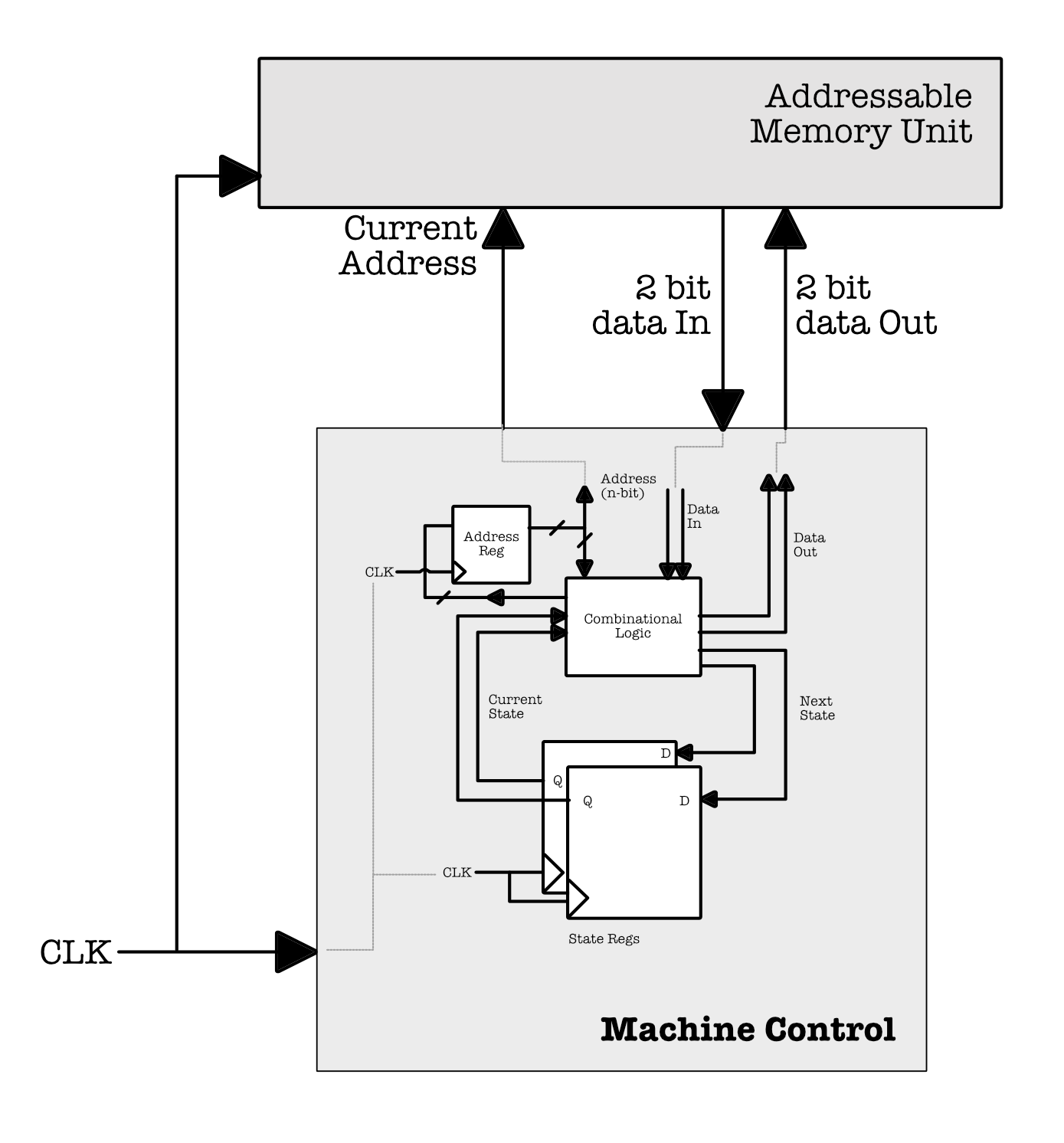 The diagram above shows a rough schematic on how we can realise the abstract concept of a Turing Machine with a specification that does increment by building a (non-programmable) physical machine that can only do this one task.
The Halting Function
This section is difficult, and is solely written for a deeper understanding about uncomputable function. You are not required to derive this proof during exams.
The simpler explanation
The Halting Function
A function that determines whether Turing Machine that’s run with specification \(K\) will halt when given a tape containing input \(j\). What is a “halt”? For example, we can write a program as an input to our machine (computers).
The program:
print("Hello World")halts, while this program:while(True): print("Hello World")does not halt.
The Halting function is uncomputable. Here’s why it is uncomputable:
-
Suppose
HALTexists: We assume we have a program calledHALTthat can analyze any other program,P, with some input,X, and tell us ifPwill stop (halt) or run forever (loop) when given that input. - Create a Paradox Program (
PARADOX): Now, let’s write a new program,PARADOX, that does something unusual:- It uses
HALTto check if itself (PARADOX) will halt when given its own code as input. PARADOXis set up to do the opposite of whatHALTpredicts:- If
HALTsaysPARADOXwill halt, thenPARADOXgoes into an infinite loop. - If
HALTsaysPARADOXwill loop, thenPARADOXhalts immediately.
- If
- It uses
- The Contradiction:
- If
HALTsays thatPARADOXhalts, thenPARADOXshould loop (by its own instructions), which contradictsHALT’s prediction. - If
HALTsays thatPARADOXloops, thenPARADOXshould halt immediately, again contradictingHALT’s prediction.
- If
This contradictory setup shows that HALT cannot make a correct prediction about every possible program, including PARADOX. In other words, this paradox proves that a universal HALT program cannot exist, because it would lead to logical contradictions when applied to programs that reference themselves.
This self-referential concept is similar to a paradox in natural language, like “This statement is false.” If the statement is true, then it must be false, but if it’s false, it must be true. The Halting Problem uses a similar type of self-reference to show that a universal halting-decider is impossible.
The in-depth explanation
Let’s symbolise the halting function (suppose it exists) as \(f_H(K,j)\), and give it a definition:
\[\begin{aligned} f_H(K,j) = &1 \text{ if } T_K[j] \text{ halts}\\ &0 \text{ otherwise} \end{aligned}\]If \(f_H(K,j)\) is computable, then there should be a specification \(H\) that can solve this.
Lets symbolise a Turing machine with this specification as \(T_{H}[K,j]\).
Now since there’s no assumption on what \(j\) is, \(j\) can be a machine (i.e: program) as well. So the function \(f_H(K,K)\) should work as well as \(f_H(K,j)\).
In Laymen Terms
Inputting a machine to another machine is like putting a program as an input to another program. Lots of programs do this: compilers, interpreters, and assemblers all take programs as an input, and turn it into some other program. Remember, \(T_K\) is basically a Turing machine with specification \(K\). We can have a Turing machine that runs with specification \(K\) with input that is its own specification (instead of another input string \(j\), symbolised as \(T_K[K]\).
With this new information (and assumption that \(f_H(K,j)\) is computable), lets define another specification \(H'\) that implements this function:
\[\begin{aligned} f_{H'}(K) = f_{H}(K, K) = &1 \text{ if } T_K[K] \text{ halts}\\ &0 \text{ otherwise} \end{aligned}\]Lets symbolise a Turing machine with this specification as \(T_{H'}[K]\) (there’s no more \(j\)).
Finally, if we assume that \(f_{H'}(K)\) is computable, then we can define another specification \(M\) that implements the following function:
\[\begin{aligned} f_M(K) = &\text{loops forever} \text{ if } (f_{H'}(K)== 1) \\ &halts \text{ otherwise} \end{aligned}\]A Turing machine running with specification M is symbolised as \(T_M[K]\).
Let’s Pause!
- \(K\) is an arbitrary Turing Machine specification, \(T_K\) is a machine built with this specification.
- \(j\) is an arbitrary input
- \(H\) is the specification that “solves” the halting function: \(f_H(K,j)\). \(T_H\) is a machine built with this specification.
- \(H'\) is the specification that “solves” a special case of halting problem: \(f_{H}(K,K)\), i,e: when \(T_K\) is fed \(K\) as input (instead of \(j\)). \(T_{H'}\) is a machine built with this specification.
- \(M\) is the specification that tells the machine running it to loop if \(f_{H'}\) returns 1, and halts otherwise. \(T_{M}\) is a machine built with this specification.
To summarise, \(T_M\) loops if \(T_K[K]\) halts (hence the output of \(T_{H'}[K]\) is 1), and vice versa.
Now since \(K\) is an arbitrary specification, we can make \(K=M\), and fed the function \(f_M\) with itself:
\[\begin{aligned} f_M(M) = &\text{loops forever} \text{ if } (f_{H'}(M)== 1) \\ &halts \text{ otherwise} \end{aligned}\]Running \(T_M[M]\) will call these chain of events. We explain it in terms of “function calls” instead of Turing machine running (although they are equivalent) because it may be easier to understand.
When we call \(f_M(M)\) (running \(T_M[M]\)), it needs to call \(f_{H'}(M)\) (run \(T_{H'}[M]\)) because it depends on the latter’s output. \(f_{H'}(M)\) depends on \(f_H(M,M)\): the original halting function that outputs 1 if \(T_M[M]\) halts, and 0 otherwise. That means, we need to call \(f_H(M, M)\) to find out its output, so that \(f_{H'}(M)\) can return. Calling \(f_H(M, M)\) requires us to run a Turing Machine with specification \(M\) on input \(M\) (run \(T_M[M]\) for another time), identical with what we did in step (1) above (just like recursive function call here).
Now here is the contradiction:
- If the running of \(T_M[M]\) from step (4) halts, then it will cause \(T_{H′}[M]\) to return \(1\). If \(T_{H′}[M]\) returns 1, then the running of \(T_M[M]\) from step (1) loops forever.
- But, if the running of \(T_M[M]\) from step (4) loops forever, then it will cause \(T_{H′}[M]\) to return \(0\). If \(T_{H′}[M]\) returns 0, then the running of \(T_M[M]\) from step (1) halts.
Neither can happen.
Therefore, specification \(M\) does not exist and it is not realisable. And by extension, everything falls apart: specification \(H'\) and \(H\) do not exist either. This means that \(f_H(K,j)\) is not computable.
Still Confused?
That’s okay. This video contains some simple animation to help you understand, give it a try.
Simple Intuition
By intuition, we know we can’t build such crash detection machine because there are very simple programs for which no one knows whether they halt or not. For example, the following Python program will HALT if and only if Goldbach’s conjecture is false.
Goldbach’s Conjecture
Every even natural number greater than 2 is the sum of two prime numbers.
It’s so easy to write this program in Python,
def isprime(p):
    return all(p % i for i in range(2,p-1))

def Goldbach(n):
    return any( (isprime(p) and isprime(n-p))
           for p in range(2,n-1))

n = 4
while True:
    if not Goldbach(n): break
    n+= 2
However, we won’t know if this program will ever stop or not. You may need to run it until forever ends (which is impossible).