 50.002 CS
- Overview
- Software: Our Abstraction Strategy
- Assembler
- Beta Extended Macroinstructions
- Interpreter vs Compiler
- Compiling Expressions
- Summary
- Next Steps
- Appendix
50.002 Computation Structures
Information Systems Technology and Design
Singapore University of Technology and Design
Assemblers and Compilers
You can find the lecture video here. You can also click on each header to bring you to the section of the video covering the subtopic.
Detailed Learning Objectives
- Explain the Concept of Abstraction in Software Engineering
- List out the definition and importance of abstraction in software engineering and computer science.
- Explain how abstraction helps in managing complexity by hiding unnecessary details and allowing focus on higher-level problems.
- Explain Software Tools for Abstraction
- Examine different tools and software that provide layers of abstraction in computing, including assemblers, compilers, and interpreters.
- Explain the role of operating systems and applications in abstracting resource management, security details, and other underlying complexities.
- Explain Various Language Abstraction Levels
- Explain the progression from machine language to high-level programming languages through assembly language, and how each level abstracts the complexity of the underlying hardware.
- Explain how language constructs like subroutines, modules, and polymorphism further abstract programming tasks.
- Experiment with Assemblers and Their Role in Programming
- Define what an assembler is and how it functions as a primitive compiler to translate assembly language into machine language.
- Outline the Beta UASM and its role in providing a symbolic representation for the Beta assembly language.
- Differentiate Between Interpreters and Compilers
- Compare and contrast interpreters and compilers in terms of how they execute high-level languages.
- Explain the trade-offs between these tools in terms of execution speed, error detection, and ease of debugging.
- Translate High-Level Constructs to Machine Language
- Practice translating high-level language constructs, such as variable declarations, arrays, conditionals, and loops, into Beta machine language.
- Assess the strategies for optimizing the translation process to reduce instruction count and memory operations.
These objectives aim to equip us with a deep understanding of how software abstraction layers work to simplify programming and enhance the usability of computing systems. We will gain practical skills in using assemblers and understanding the transformation of high-level constructs into executable machine code.
Overview
The goal of this chapter is to help us understand how to improve the programmability of the \(\beta\) (or any ISA in general). The \(\beta\) machine language is encoded into 32-bit instructions each.
For example, the 32-bit ADD instruction is:
100000 | 00100 | 00010 | 00011 | 00000000000
The \(\beta\) understands it as: Reg[R4] = Reg[R2] + Reg[R3]
However, most of us would prefer to write: ADD(R2, R3, R4), or even a = b+c because we couldn’t care less which registers are used as long as the CPU can add two variables together and produce the correct result.
We need to improve the programmability and usability of our machine by providing abstraction, that is so that we can program (e.g: write code) and/or use the machine in an easier way by removing irrelevant data, hence allowing us to concentrate on one issue at a time.
We can do this by writing various softwares that allow us to abstract some details so that it is easier to fulfil our tasks.
Software: Our Abstraction Strategy
Abstraction
Abstraction is a fundamental concept in software engineering and computer science. It refers to process of removing physical, spatial, or temporal details to allow us to focus our attention on matters of greater importance.
We can engineer various softwares to provide abstraction in a computer system. A central form of abstraction in computing is the language abstraction.
Language Abstraction
Language abstraction is a generational development of programming languages from the machine language to the assembly language and finally to the high-level language. Each stage can be used as a stepping stone for the next stage.
We can also create new abstraction within a programming language, such as subroutines, modules, software components, polymorphism, and so on.
Layers of Software Abstraction
Basic Layer
This layer includes compilation tool softwares such as assemblers, interpreters and compilers:
- Assemblers and Interpreters: hides bit-level representations, hex locations, and binary values
- Compilers: hides machine instructions, registers, machine architecture
Higher Layers
This layer includes interpretive software tools such as the Operating System and certain Applications (web browser, integrated development environment (IDE), game engines, etc):
- Operating System: hides resources (memory, CPU, I/O devices) limitations and details.
- Applications: hides local parameters, network location, security details, etc.
Assembler
Definition
An assembler is technically a program for writing programs. It also can be called as a primitive compiler.
Its job is to parse a symbolic language (assembly language) used to represent instructions for the CPU to execute.
beta.uasmandbsim
bsimis the simulator for our toy Beta CPU, and the simulator part only understands machine language in terms of 1s and 0s (the 32-bit instructions loaded at each CLK cycle).bsimalso incorporates an assembler, which is a program that converts text files into binary memory. It utilisesbeta.uasmwhich contains all symbol definitions for all the registers and macro definitions for Beta instructions.If you haven’t done so, you can download both from here.
The assembler enables us to write programs for our Beta CPU symbolic language called beta assembly language for our bsim to execute.
UASM
UASM is MIT’s 6.004 Micro Assembly Language. It describes the Beta instructions to the built-in assembler in bsim.
In order to write a programs that can be runnable by our Beta CPU in bsim conveniently, we need a UASM:
- A symbolic language (UASM) for representing strings of bits of instructions.
- A Program for translating UASM source code into binary.

A UASM source file contains (in symbolic text) values of successive bytes to be loaded into memory. We can define various things in UASM source file. Refer to beta.uasm:
- It reads arithmetic expressions and evaluates them to produce 8-bit values, which it then adds sequentially to the array of bytes which will eventually be loaded into the Beta’s memory.
- UASM supports several useful language features like symbols and labels that make it easier to write assembly language programs.
- Symbols and labels let us give names to particular values and addresses.
- Macros let us create shorthand notations for sequences of expressions that, when evaluated, will generate the binary representations for instructions and data.
Read the bsim Documentation
Please read the
bsimdocumentation to know more about the syntax of the Beta assembly language.You can head to the Appendix if you would like to know more about how and assembler work.
The next few sections explains the syntax that’s acceptable by the Beta Assembler. We will use the same syntax in exams and problem sets.
Symbols
Symbols can be defined using the = sign allows us to “rename” basic values (like defining variables):
x = 0x1000
y = 0x1004

R0 = 0
R1 = 1
R2 = 2

ADDC(R0, x, R1) | equivalent to ADDC(0x0, 0x1000, 0x1)
ADDC(R1, y, R1) | equivalent to ADDC(0x1, 0x1004, 0x1)
ADDC(R1, R2, R3) | not an error, equivalent to ADDC(0x1, 0x2, 0x3)
The dot .
The . is a special symbol which dictates where next byte address to be filled in memory is.
. = 0x100
ADDC(R0, 3, R1) | means to put (load) this instruction at address 0x100
It can be used in these contexts:
As regular instruction loading address:
.include beta.uasm

. = 0x000
ADDC(R1,3,R1) | address 0
SUBC(R1,10,R2) | address 4
ST(R1, j, R31) | address 8
BEQ(R31, end, R31) | address 12
j: LONG(5)


. = 0x100
end: BEQ(R31, 0, R1) | address 256
The above writes BEQ(R31, 0, R1) at address 0x100.
As label replacement:
.include beta.uasm

. = 0x000

ADDC(R1,3,R1) | address 0
SUBC(R1,10,R2) | address 4
ST(R1, j, R31) | address 8
BEQ(R31, . - 12, R31) | address 12

j : LONG(5)
This causes the BEQ to branch to this current address (recall “dot” means “here”, this byte’s address) - 12, which is 12 (BEQ's address) - 12 = 0, resulting in address 0 as the branch destination. It is equivalent to BEQ(R31, 0x0, R31).
LONG(x)
This is a macro (shorthand) to convert x into 32-bit word. See this section.
To populate memory content:
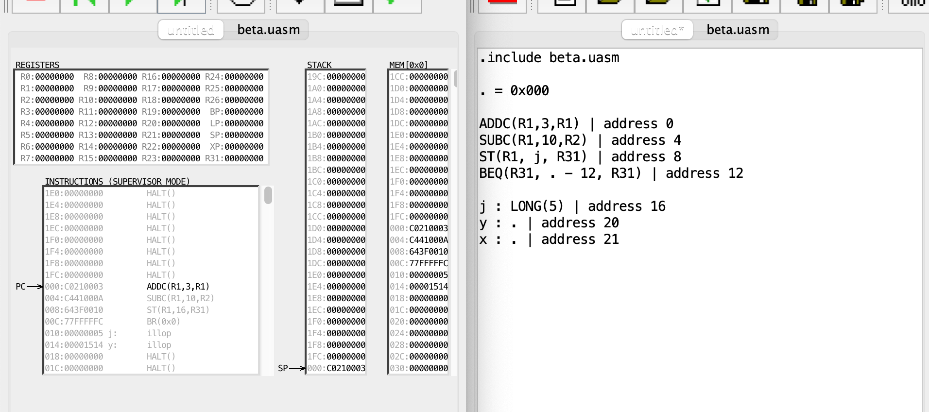
.include beta.uasm

. = 0x000

ADDC(R1,3,R1) | address 0
SUBC(R1,10,R2) | address 4
ST(R1, j, R31) | address 8
BEQ(R31, . - 12, R31) | address 12

j : LONG(5) | address 16
y : . | address 20
The content of Mem[16] is word (32-bits) 0x00000005, and the content of Mem[20] is byte 0x14.
If we do another one:
.include beta.uasm

. = 0x000

ADDC(R1,3,R1) | address 0
SUBC(R1,10,R2) | address 4
ST(R1, j, R31) | address 8
BEQ(R31, . - 12, R31) | address 12

j : LONG(5) | address 16
y : . | address 20
x : . | address 21
We would have Mem[21] as byte 0x15 (which is 21). That means we are simply filling the content of address 20 and 21 as the address value itself in bytes.
If it is still confusing, compile it in bsim.
Labels
Labels are symbols that represent memory addresses. It is defined using the :. For instance, begin_loop is a label.
. = 0x100
ADDC(R31, 3, R1) | means to put (load) this instruction at address 0x100

begin_loop : SUBC(R1, 3, R1)  | begin_loop is a label, which value is the address this SUBC instruction
BEQ(R1, begin_loop, R31) | loop to the SUBC instruction above if content of R1 is 0, else HALT()
HALT()
Count the Address
ADDCis loaded at address0x100. SinceADDC’s length is 4 bytes,SUBCis loaded at the subsequent address :0x104.
Beta Extended Macroinstructions
We augment the basic Beta instruction set with the following macros, making it easier to express certain common operations:
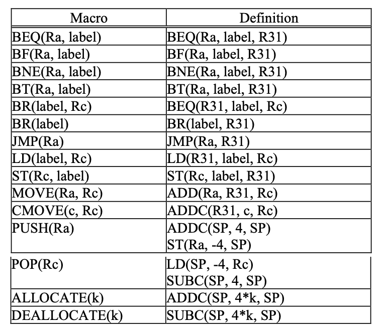
We will use these extended macroinstructions in exam and problem sets.
HALT()
This is a special instruction that simply cause the Beta CPU simulator to stop execution. You can treat this as a stop instruction.
Interpreter vs Compiler
Some higher level languages, like Java and C/C++ have to be compiled first using its respective compilers (javac for Java or GCC for C/C++), resulting in an executable (a sequence of binary instructions directly understandable by the CPU).
Compilers typically go through sophisticated steps of analysing the entire high-level source code to produce an optimized set of instructions for the machine. We will not be able to execute the program if the compiler meets an error, hence making it comparatively harder to debug. It slows down program development but it will result in faster execution.
Other languages like Python and Ruby are interpreted. The interpreter for these languages execute the program directly, often by translating each line of code into a sequence of one or more standard subroutines, and finally into machine code.
There’s comparably less analysis of source code done, and the interpreter translates the program on the fly. It will execute the program until the first error is met, hence debugging will be comparatively easier than debugging compiled languages.
For instance, you cannot compile a C program with such error, and no Hello World! will be printed out.
//test.c
#include <stdio.h>
int main() {
   // printf() displays the string inside quotation
   printf("Hello World!");
   asdfsadf // some deliberate error
   return 0;
}
In comparison, the following Python program will still print Hello World! before terminating in a syntax error:
# test.py
print("Hello World!")
asdfasdf # some deliberate error
Compiling Expressions
In this course, we will not dive into how compilers, assemblers, or interpreters work in too much detail. In fact, we are going to hand compile the high-level language (we will use C) ourselves into \(\beta\) assembly (and then hand assemble them into the binary executable).
Don’t worry. Compilation to unoptimized code is pretty straightforward. You won’t be required to write C-code either, only to read them.
There are several rules to keep in mind in order to do this well:
- Variables are assigned to memory locations and accessed via
LDandST - Operators (
+,-,*,/,>, <, ==, etc) translate to ALUOP- Small constants translate to
c(literal-mode) ALU instructions - Large constants must be loaded to registers first
- Small constants translate to
- Conditionals and loops involve
BEQorBNE - Function return involve
JMP
Let’s dive into simple examples to make this clearer.
To aid your learning, copy each snippet to bsim and observe the instruction execution step by step.
Example 1: Basic Variable Declarations
C Code:
int x,y; // initialize x, y
x = 20; // fill x with 20

// other code
// then eventually we use  y
y = x + 5;
Translates to the following \(\beta\) assembly code:
.include beta.uasm
ADDC(R31, 20, R9) 	| populate 20 to R9, selection of R9 is arbitrary
ST(R9, x, R31)		| store 20 at x

||| assume other code
||| we can't assume that R9 still contains x so we need to reload it
LD(R31, x, R1)		| load the content of memory address x to R1
ADDC(R1, 5, R0)		| now that '20' is in R1, add it with 5, store it at R0
ST(R0, y, R31) 		| store the result (at R0) to location y
HALT()

x : LONG(0)	| label x points to where 20 is stored
y : LONG(0)		| label y points to where 0 is stored
Example 2: Arrays
C Code:
int x[5];
x[0] = 12;
x[1] = 13;
x[2] = x[0] + x[1];
Translates to the following \(\beta\) assembly code:
.include beta.uasm

||| Populate contents of array x
ADDC(R31, 12, R0)	| supposed content of x[0]
ST(R0, x)			| store '12' in R0 at address x
ADDC(R31, 13, R1)	| supposed content of x[1]
ADDC(R31, 4, R2) 	| index 1 (x[1] -> x+4)
ST(R1, x, R2)    	| store '13' in R1 at address (x+4)
ADD(R0, R1, R3) 	| x[0] + x[1] = 25
ADDC(R31, 8, R2) 	| index 2 (x[2] -> x+8)
ST(R3, x, R2) 		| store '25' in R3 at address (x+8)
HALT()

x : .
Example 3: Conditionals
C Code:
x = 128
number = 5; // Change this value to test different cases

// If-else condition to check the number
if (number > 0) {
	x = x + 1
} else if (number < 0) {
	x = x - 1
} else {
	x = 1
}
Might translate to the following \(\beta\) assembly code:
.include beta.uasm

LD(R31, x, R1) | put x to R1
LD(R31, number, R2) | put number to R2

CMPLE(R2, R31, R3) | check if number is <= 0
BEQ(R3, number_gt_zero, R31)
CMPEQ(R2, R31, R3) | check if number is == 0
BEQ(R3, number_lt_zero, R31)
| if reach here, number is zero
ADDC(R31, 1, R1)  | set 1 to x
BR(halt)

number_gt_zero:
ADDC(R1, 1, R1) | x = x + 1
BR(halt)

number_lt_zero:
SUBC(R1, 1, R1) | x = x - 1
BR(halt)

halt:
ST(R1, x, R31)
HALT()

number : LONG(20)
x : LONG(128)
Example 4: Loops
C Code:
int n = 20;
int r = 1;

while (true){
	if (n <= 0) break;
	r = r*n;
	n = n-1;
}
Might translate to the following \(\beta\) assembly code:
.include beta.uasm

LD(R31, n, R1)
LD(R31, r, R2)

check_while: CMPLT(R31, R1, R0)	| compute whether n > 0
BNE(R0, while_true, R31) | if R0 != 0, go to while_true
ST(R2, r, R31)			 | store the result to location 'r'
ST(R1, n, R31)			 | store the result to location 'n'
HALT()

while_true: MUL(R1, R2, R2) | r = r*n
SUBC(R1, 1, R1) 			| n = n-1
BEQ(R31, check_while, R31) 	| always go back to check_while

n : LONG(20)
r : LONG(1)
Summary
You may want to watch the post lecture videos here:
Here are the key points from this notes:
- Symbolic Language and UASM: UASM (Universal Assembler) is used for representing strings of bits in instructions. It allows for defining variables and instructions in a human-readable format that can be easily converted into binary.
- Symbols and Labels: These are used in UASM to define constants and memory addresses. Symbols simplify the code by allowing the use of names instead of numeric addresses or values.
- Macroinstructions: Macroinstructions simplify assembly language programming by allowing more complex operations to be performed with simpler commands. These macros help abstract the underlying complexity of machine instructions.
- Compilers and Interpreters: Compilers analyze and translate the entire source code into executable machine code, which tends to make debugging harder but execution faster. Interpreters, on the other hand, translate and execute code on the fly, which simplifies debugging.
- Compiling Expressions: We compile simple expressions into assembly language, focusing on variable memory locations, ALU operations, array creation, and control flow constructs like conditionals and loops.
These concepts are crucial for understanding how software is developed and executed on hardware, providing a practical framework for us to understand the integration of software and hardware through the compilation process.
Next Steps
Note that there are a lot of ways to translate higher level language into a lower level language (various optimisations and code rearrangement done, etc). The examples given above are not necessarily the most optimised way but it’s probably the most straightforward (easiest) way to hand-compile a higher-langauge expression.
We should ask ourselves:
- Is it possible to reduce the number of instructions?
- Is it possible to reduce the amount of
LDandST?
The examples above are also not exhaustive. There are several undiscussed parts:
- How do we reuse boilerplate code?
- How do we write functions? Declare structures?
- Where do we keep local variables if the number of local variables exceeds the number of registers?
- How do we discard local variables and define scoping?
We will address some of these questions in the next chapter.
Creating an optimised compiler is not a trivial task. For now, don’t worry too much about it. We simply only need to hand assemble C into \(\beta\) assembly language, and have a general idea on what a compiler, interpreter, and assembler are for – that is to enhance the programmability of a computer by providing software abstraction. If you’re interested, you can choose to take compiler related electives in the future.
Appendix
This section gives more elaboration about beta.uasm assembler implementation.
Basic Values Loading Into Memory
Basic values comprise of Decimals, binary (with 0b prefix), and hexadecimal (with 0x prefix). All these will be loaded (from low to high address) as 1 byte each, separated by spaces.
For example, if we have 4 different values to be stored: 5, then 6, then 7, then 8, it will be stored as 08 07 06 05 as a consecutive 8 bytes in memory. 05 gets the lowest address, and 08 gets the highest address. Anything that requires more than 1 byte to represent/store, such as values like: 256 257 258 259 will be truncated into 1 byte only, and resulted as the following in memory (only remainder left): 03 02 01 00. This is why it is important to establish the concept of data type.
A typical ASCII char takes 1 byte per character and an int data type occupies 4 bytes.
Assembler Macroinstructions
Macroinstructions parameterized abbreviations, also known as aliases or shorthands. There are plenty of Beta assembly language macros supported in bsim and you have to read the documentation to find out more.
There are two important basic macros in particular: WORD and LONG which allows us to assemble input x that is more than 256 into longer streams of bytes
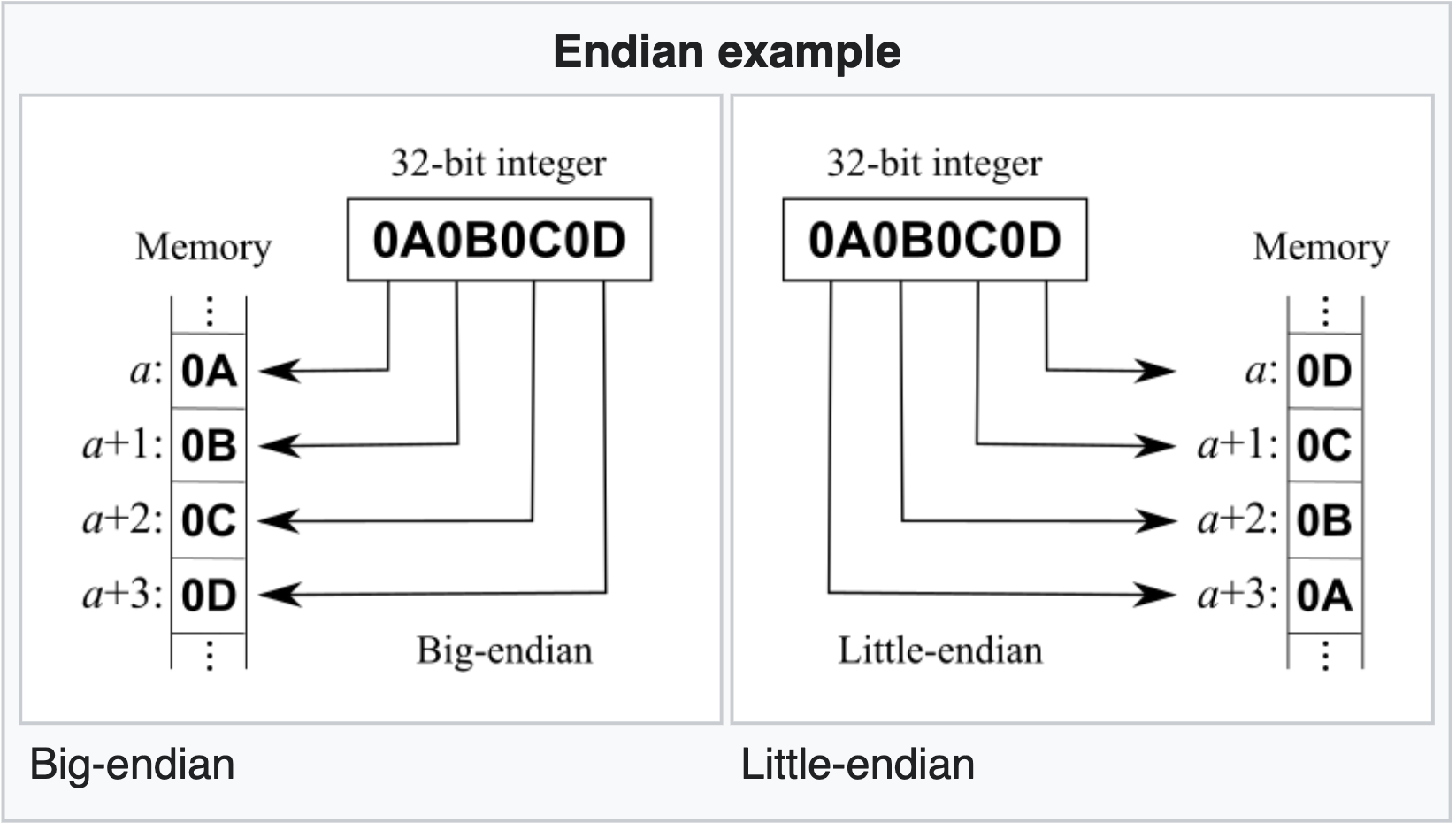
- There are two ways of storing bytes in memory: the little endian format where lowest byte stored at the lowest address and vice versa, and the big endian format where the highest byte is stored at the lowest address and vice versa.
- The \(\beta\) CPU follows the little-endian format
This diagram (taken from here) represents the differences between the two. In short, it’s just how we choose to store our data. Since the \(\beta\) CPU follows the little-endian format. It loads data byte-by-byte to the memory, and the least significant byte of our data into the memory with the lowest address.
Here is the relevant implementaiton of WORD and LONG in beta.uasm.
.macro WORD(x) x%256 (x/256)%256
.macro LONG(x) WORD(x) WORD(x >> 16)
More complex \(\beta\) instructions are also created by writing these convenient macroinstructions. For example, we want to load the following instruction into memory:
OPCODE  Rc	  	Ra    	c
110000 	00000 	11111	1000 0000 0000 0000
Notice that the above is an ADDC instruction, to add contents of R31 with -32768 and store it at R0.
Without any macros, we would need to load them in the different order (remember, the Beta follows little-endian arrangement):
00000000    10000000    00011111    11000000
|                       |  |        |     |
|                       |  |        |     |-Rc[4:3]
|                       |  |-Ra[4:0]|
|-c[15:0]               |-Rc[2:0]   |-OPCODE[5:0]
With this arrangement, OPCODE=110000 is stored at a higher address than Rc, and Rc=00000 is at a higher memory address than Ra, and 16-bit constant c is at the lowest memory address of the entire word.
It should be obvious that writing the above instruction in little-endian compatible form is so unintuitive. We need to chop the original instruction into 1 byte chunks and “load” them from right to left so they’re stored from lowest to highest memory location to follow the little-endian format.
With a slight improvement from macro LONG, we can write them naturally as:
LONG(0b11000000000011111000000000000000)
Better yet, we can define a macro called betaopc and ADDC that relies on the former:
.macro betaopc(OP,RA,CC,RC) {
	.align 4
	LONG((OP<<26)+((RC%32)<<21)+((RA%32)<<16)+(CC % 0x10000))
}
.macro ADDC(RA,C,RC) betaopc(0x30,RA,C,RC)
Then we can use the ADDC symbol to easily to load our instruction above in a more intuitive way:
ADDC(R15, -32768, R0)
In summary, the file beta.uasm given for your lab provides support for all \(\beta\) instructions so that we can write instructions for \(\beta\) in a much more intuitive way without caring about the details on how to load these values properly into memory (abstraction provided). We can now finally write instructions using symbols (called macros) like ADD, SUB, MUL, JMP, CMPLEC, BEQ, BNE, and more instead of writing it in machine languages thanks to this assembler.
| BETA Instructions:

|| OP instructions (other OP like SUB, CMPLE, etc should work the same)
.macro ADD(RA,RB,RC) betaop(0x20,RA,RB,RC)
.macro AND(RA,RB,RC) betaop(0x28,RA,RB,RC)
.macro MUL(RA,RB,RC) betaop(0x22,RA,RB,RC)

|| OPC instructions (other OPC like SUBC, CMPLEC, etc should work the same)
.macro ADDC(RA,C,RC) betaopc(0x30,RA,C,RC)
.macro ANDC(RA,C,RC) betaopc(0x38,RA,C,RC)
.macro MULC(RA,C,RC) betaopc(0x32,RA,C,RC)

...
|| Memory Access instructions
.macro LD(RA,CC,RC) betaopc(0x18,RA,CC,RC)
.macro ST(RC,CC,RA) betaopc(0x19,RA,CC,RC)
.macro LDR(CC, RC) betabr(0x1F, R31, RC, CC)


|| Transfer Control instructions
.macro betabr(OP,RA,RC,LABEL)	betaopc(OP,RA,((LABEL-.)>>2)-1, RC)
.macro JMP(RA, RC) betaopc(0x1B,RA,0,RC)
.macro BEQ(RA,LABEL,RC) betabr(0x1D,RA,RC,LABEL)
.macro BNE(RA,LABEL,RC) betabr(0x1E,RA,RC,LABEL)
Endianess
Suppose we want to store the word 0xDEADBEEF to memory address 0x0. We start by loading 0xEF to address 0x0, then 0xBE to address 0x1, and so on. This is so tedious to do. Using the macro: LONG(0xDEADBEEF) has the same effect as storing: 0xEF 0xBE 0xAD 0xDE to memory in sequence from low to high memory address, resulting in the following:
| Address | 0x0 | 0x1 | 0x2 | 0x3 |
|---|---|---|---|---|
| Content | 0xEF | 0xBE | 0xAD | 0xDE |
If one were to store 0xDEADBEEF in big-endian format, it will result in:
| Address | 0x0 | 0x1 | 0x2 | 0x3 |
|---|---|---|---|---|
| Content | 0xDE | 0xAD | 0xBE | 0xEF |
bsim Memory Address Display
Our bsim.jar program displays the memory address the other way around, that is high address on the left and low address on the right, so our little-endian format in \(\beta\) looks like the big-endian format for easy debugging:
| Address | 0x3 | 0x2 | 0x1 | 0x0 |
|---|---|---|---|---|
| Content | 0xDE | 0xAD | 0xBE | 0xEF |