 50.005 CSE
- Stuck in the Queue
- Battle of the Bandwidth
- A Packet’s Journey
- The Mistaken Sprint
- Sleepy Socket
- Fast-in Slow-out
- Packets Keep Coming, But Nobody’s Home (Yet)
- Bits on the Move with a Ticking Timeout
- The Calm Before the Queue
- The Idle Interface
- The Overstuffed Switch
50.005 Computer System Engineering
Information Systems Technology and Design
Singapore University of Technology and Design
Natalie Agus (Summer 2025)
Network Performance
Stuck in the Queue
Background: Components of Network Delay
Recall that network delay is made up of four components:
- Processing delay: time to examine and route the packet at each hop
- Queuing delay: time spent waiting in buffers before transmission
- Transmission delay: time to push the packet onto the link
- Propagation delay: time for bits to travel through the medium
Each hop in a network path contributes to total delay differently depending on hardware, load, and distance. Understanding which delay dominates at each point helps identify bottlenecks and optimize performance.
Scenario
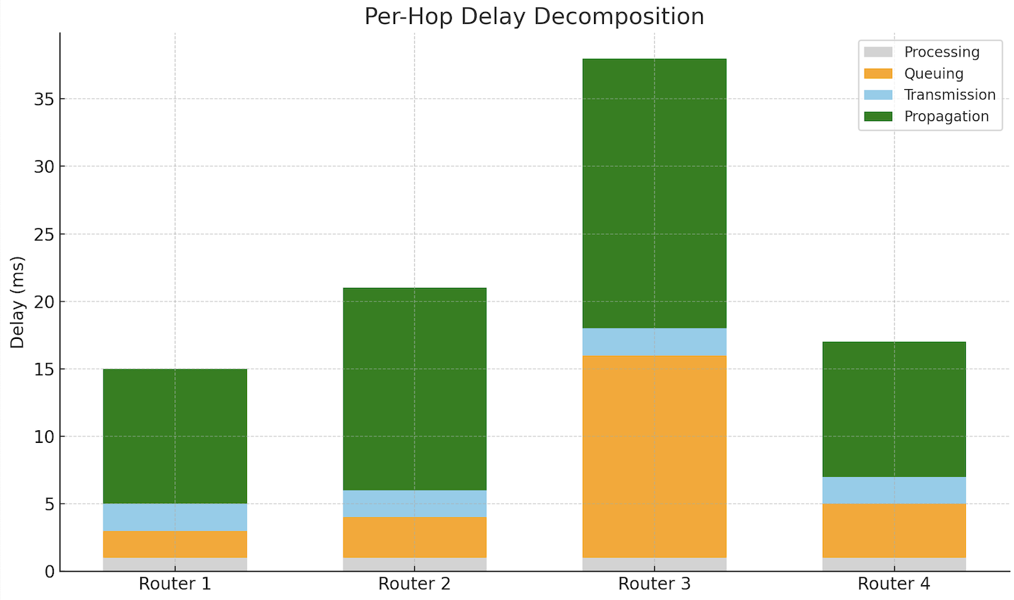
A packet travels across four routers to reach a destination. The network includes a mix of low-latency fiber and high-load shared links. The student is shown a timeline diagram as shown below where each hop is broken into segments of processing, queuing, transmission, and propagation delay. The queuing segment grows significantly at one hop, causing total delay to spike:
Answer the following questions:
- How can you tell which delay is dominating at a hop?
- What conditions cause queuing delay to grow?
- Why does processing delay usually remain constant?
- What network behaviors could flatten or steepen the delay curve?
Hints:
- Queuing depends on arrival rate vs. service rate
- Processing time depends on router speed and configuration
- Transmission is based on packet size and link speed
- Propagation depends only on physical distance
- Bursts or congestion affect queuing the most
You can tell which delay dominates at a hop by observing the relative size of each component. A tall queuing bar, for example, indicates congestion at that router.
Queuing delay grows when packets arrive faster than they can be forwarded. This happens during congestion, bursty traffic, or near link saturation.
Processing delay is typically short and predictable. Modern routers can examine and forward packets in microseconds unless overloaded.
Delays can be minimized by spreading out traffic, upgrading hardware, or rerouting around congested paths. Adaptive queue management and traffic shaping also help smooth out spikes in delay.
The Hidden Layer
Background: The 5 Layers
Network performance depends not only on bandwidth and propagation, but also on which layers of the system introduce delay. The Internet is modeled as a 5-layer architecture:
- Application: protocols like HTTP, FTP
- Transport: TCP, UDP
- Network: IP
- Link: Ethernet, Wi-Fi
- Physical: cables, signals
The operating system is responsible for parts of layers 2–4. The transport layer, including socket buffers and TCP congestion control, is implemented inside the OS kernel. The network layer is handled by routing logic and packet forwarding. The link layer involves device drivers and network interface queues. Delays at these OS-managed layers (such as socket buffering or driver queuing) contribute to total response time but are often overlooked by application developers.
Scenario
An HTTP request from a user appears slow. A network diagnostic shows low propagation delay and high bandwidth. However, further investigation reveals the OS socket buffer is full, and the network interface queue is also growing.
Answer the following questions:
- Which network layers are managed by the operating system?
- What types of delay can occur inside the OS kernel?
- Why does a full socket buffer introduce delay even when the network is fast?
- What tools or measurements help isolate OS-induced delay?
- How can understanding layer boundaries improve performance debugging?
Hints:
- Layers 2–4 interact with kernel code
- Socket buffers and interface queues reside in the OS
- Application-layer delays may result from kernel-side queuing
- Tools like
netstat,ss, ortcpdumpcan observe kernel behavior- Not all delay is caused by the external network
The operating system manages the transport, network, and link layers. This includes socket buffers (transport), routing decisions (network), and driver-level queues (link).
Delays in the OS can occur when socket buffers fill up, when packets wait in the kernel queue before transmission, or when the NIC is busy and packets back up in driver queues. These are all forms of queuing delay.
When the socket buffer is full, the application cannot send more data until the kernel sends and frees space. Even if the physical network is fast, the backlog in the OS adds delay to the send path.
To observe these delays, tools like netstat or ss can show socket buffer usage, while tcpdump or interface statistics reveal packet queuing or drops. These help identify delays introduced before packets even leave the machine.
Understanding which layers the OS controls helps developers trace performance problems more accurately. It separates network-induced delays from software bottlenecks inside the system.
Battle of the Bandwidth
Background: Bottleneck Links
In multi-hop networks, the bottleneck link (the one with the lowest bandwidth) determines the maximum throughput along a path. To choose the best path, we must compute:
- Transmission delay per link
- Total transmission delay for a packet
- End-to-end throughput, considering bottlenecks
Assume 1000-byte packets are sent from Host A to Host B. Ignore propagation and queuing delay.
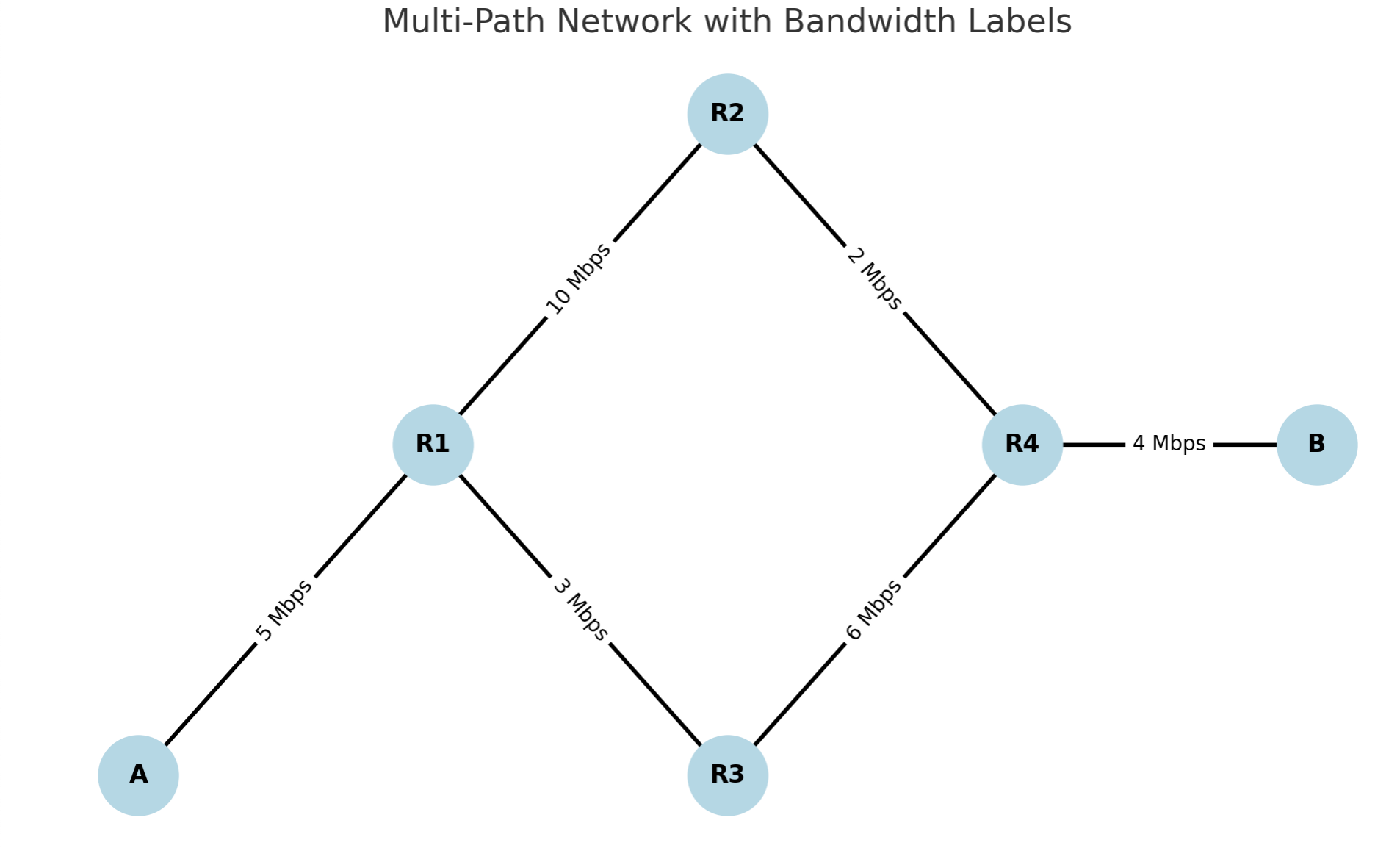
Here is the diagram of a multi-path network from A to B, passing through multiple routers with different bandwidths. Note that there are two main paths from A to B.
Scenario
Using the graph above:
- Compute the transmission delay for each link (in ms)
- For each complete path from A to B, compute:
- Total transmission delay
- Bottleneck bandwidth
- If you had to send 1000 packets, which path would complete transmission faster?
Answer the following questions:
- What are the possible paths from A to B?
- What is the transmission delay for each link?
- What is the bottleneck link for each path?
- What is the total time to send 1000 packets over each path (pipelined)?
- Which path offers higher throughput and lower latency?
Hints:
- Transmission delay = (packet size in bytes × 8) ÷ link bandwidth
- Total transmission delay = sum of all link delays
- Bottleneck = min(link bandwidths in path)
- Pipelined time = 1st packet delay + (N-1 packets × bottleneck link delay)
- The formula arises from overlapping transmissions. After the first packet finishes the full route, subsequent packets follow in a steady rhythm defined by the slowest link, just like cars exiting a car wash every X seconds after the first.
- Prefer paths with higher bottleneck and lower total delay
The two possible paths from A to B are:
- Path 1: A → R1 → R2 → R4 → B
- Path 2: A → R1 → R3 → R4 → B
Transmission delays for each link:
- A → R1 (5 Mbps): 1.6 ms
- R1 → R2 (10 Mbps): 0.8 ms
- R2 → R4 (2 Mbps): 4.0 ms
- R4 → B (4 Mbps): 2.0 ms
Total for Path 1: 8.4 ms
- A → R1 (5 Mbps): 1.6 ms
- R1 → R3 (3 Mbps): 2.67 ms
- R3 → R4 (6 Mbps): 1.33 ms
- R4 → B (4 Mbps): 2.0 ms
Total for Path 2: 7.6 ms
Bottleneck link:
- Path 1: 2 Mbps (R2 → R4)
- Path 2: 3 Mbps (R1 → R3)
Pipelined transmission time for 1000 packets:
3- Path 1: 1st packet delay + 999 × bottleneck delay = 8.4 ms + (999 × 4.0 ms) = 4004.4 ms
- Path 2: 1st packet delay + 999 × bottleneck delay = 7.6 ms + (999 × 2.67 ms) = 2674.9 ms
Conclusion: Path 2 is better. Even though it has slightly higher delay on one link, its higher bottleneck bandwidth (3 Mbps) allows much better throughput. It completes 1000-packet transfer significantly faster than Path 1.
A Packet’s Journey
Background: Pipelined Transmission
In pipelined transmission, packets are sent back-to-back while earlier ones are still in transit. This enables high link utilization but requires understanding both transmission delay and propagation delay. These two combine to form the total time a packet takes to reach the destination.
The bandwidth-delay product (BDP) tells us how many bits can be “in flight” on the link at once. A space-time diagram helps visualize how pipelining works.
In the diagram below:
- Each diagonal line represents a 1000-byte packet
- The x-axis shows direction: from sender to receiver
- The y-axis shows time in milliseconds, growing downward
- Each blue diagonal line shows a packet being transmitted and propagating from sender to receiver.
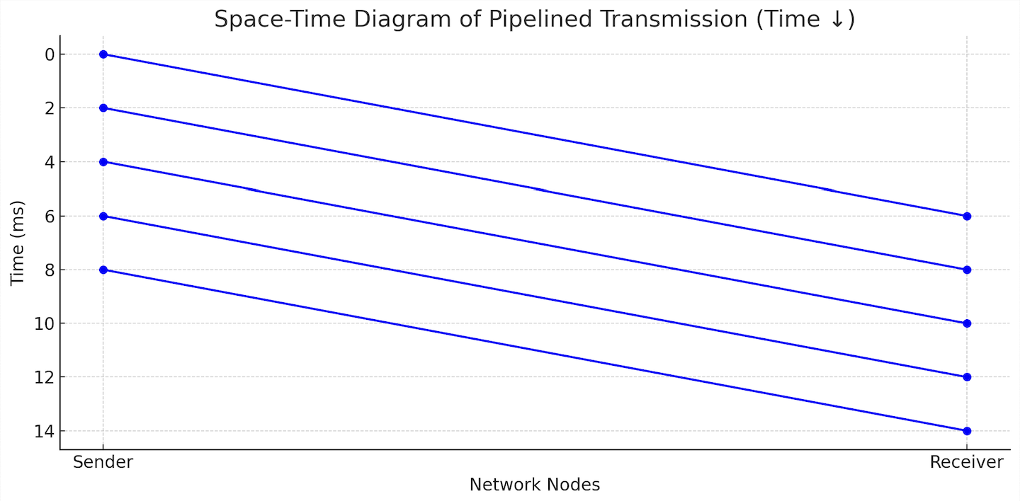
This format helps visualize packet timing in a way that aligns with packet capture tools or stack traces, where newer events appear lower.
From the diagram above, we can deduce that propagation delay is around 6ms, and transmission delay is 2ms (which makes bandwidth to be 4 Mbps).
Scenario
A host sends 5 packets (each 1000 bytes = 8000 bits) over a 1 Mbps link with 24 ms one-way propagation delay. The packets are sent back-to-back with no gaps.
Refer to the space-time diagram above for illustration, but adjust the numbers to fit this scenario.
Answer the following questions:
- What is the transmission delay per packet?
- When does the first packet arrive at the receiver?
- When does the last packet arrive?
- What is the total time to complete the transmission of all 5 packets?
- How many bits are in flight just after the third packet finishes sending?
Hints:
- Transmission delay = size ÷ bandwidth
- First packet arrives after transmission + propagation
- Each packet starts right after the previous one
- BDP = bandwidth × propagation delay
The transmission delay for each 1000-byte packet on a 1 Mbps link is:
- 8000 ÷ 1,000,000 = 8 ms
The first packet finishes transmission at 8 ms and takes 6 ms to propagate, so it arrives at:
- 8 + 24 = 32 ms
The fifth packet starts at 32 ms, finishes transmission at 40 ms, and arrives at:
- 40 + 24 = 64 ms
The total time to transmit and receive all 5 packets is from t = 0 ms to t = 64ms.
After the third packet is sent (at t = 24 ms), all three packets are in flight and have not yet arrived. The first bit of the first packet will arrive just after 24 ms. So:
- 3 × 8000 = 24,000 bits in flight
Alternatively, you can compute the bandwidth-delay product:
- 1 Mbps × 24 ms = 24000 bits. This is the maximum bits per packet in flight due to propagation
The Mistaken Sprint
Background
Transmission delay is the time it takes to push all bits of a packet onto the wire. It depends on the packet size and link bandwidth. Propagation delay is the time it takes for bits to physically travel through the medium (like fiber or copper) from sender to receiver. It depends on distance and the speed of signal propagation, not on packet size.
A common misconception is to confuse these two. In reality, a tiny packet sent across the globe has nearly zero transmission delay but significant propagation delay. Conversely, a large packet on a slow link may experience long transmission delay even over a very short distance.
Scenario
A 1000-byte packet is sent over two different links:
- Link A: 100 meters long, 1 Mbps bandwidth
- Link B: 3000 kilometers long, 1 Gbps bandwidth
Students assume Link A is faster because it is “shorter.”
Answer the following questions:
- What is the transmission delay for each link?
- What is the propagation delay for each link?
- Which link delivers the packet sooner?
- Why does distance dominate in one case, and bandwidth in the other?
- How does this distinction help when analyzing latency?
Hints:
- Transmission = size ÷ bandwidth
- Propagation = distance ÷ signal speed
- Signal speed ≈ 2 × 10⁸ m/s
- Tiny delay differences can become significant at large scale
- Always compute both components to understand total delay
Transmission delay for Link A is (1000 × 8) ÷ 1,000,000 = 0.008 seconds = 8 ms.
Propagation delay for Link A is 100 ÷ (2 × 10⁸) = 0.0000005 seconds = 0.0005 ms.
Transmission delay for Link B is (1000 × 8) ÷ 1,000,000,000 = 0.000008 seconds = 0.008 ms.
Propagation delay for Link B is 3,000,000 ÷ (2 × 10⁸) = 0.015 seconds = 15 ms.
Although Link B has nearly zero transmission delay, it takes longer overall due to propagation. Link A finishes faster because it's physically shorter, even with a slower bandwidth.
This shows that bandwidth matters most when sending large data, but distance dominates in delay-sensitive applications. Distinguishing these two helps in protocol tuning and routing decisions.
Below is a sample graph explaining the difference between transmission and propagation delay: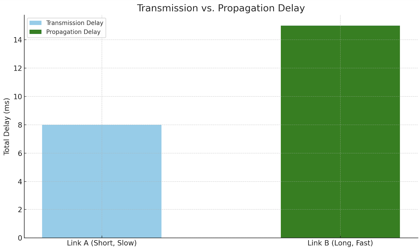
**Link A** (short distance, low bandwidth) has a large transmission delay but negligible propagation. **Link B** (long distance, high bandwidth) has almost zero transmission delay, but high propagation delay due to the physical distance.
Sleepy Socket
Background: Blocking SVC
Network communication often involves blocking system calls like read() or recv(), which wait for data to arrive. If the data has not yet reached the local socket buffer (due to propagation, queuing, or slow sender) the process is put to sleep by the OS. This frees the CPU to run other processes while the kernel waits for incoming data. When the data finally arrives, an interrupt notifies the OS, which wakes the blocked process and schedules it to resume. This mechanism ensures CPU efficiency but introduces performance sensitivity to network delay.
Scenario
A process issues read(sockfd, buf, 100) to receive 100 bytes from a remote server. The network introduces 120 ms of delay before the data reaches the socket buffer. During this time, no CPU is used, and the process is marked as sleeping.
Answer the following questions:
- Why does the OS block the process instead of spinning?
- How is this blocking behavior related to network performance?
- What role does the interrupt mechanism play in this scenario?
- When does the process resume, and how is scheduling involved?
- How can this type of delay be measured or profiled?
Hints:
- Blocking avoids wasting CPU cycles
- Sleep queues allow efficient multitasking
- Arrival of data triggers a hardware interrupt
- Wakeup is followed by re-scheduling
- Tools like
strace,perf, or timestamps can expose this delay
The OS blocks the process to avoid busy-waiting and wasting CPU resources. This is more efficient than looping continuously while checking if data has arrived.
Blocking behavior interacts with network performance because the total time the process sleeps depends on when the network delivers the data. High propagation or queuing delay increases time spent in the blocked state.
When the data arrives at the network interface, a hardware interrupt signals the OS. The driver copies the data into the socket buffer and checks if any process was blocked waiting for it.
The process is marked as runnable and placed on the scheduler's queue. It resumes when the OS chooses it to run, depending on priority and system load.
This delay can be observed using tools like strace (to trace the time spent in read()), or by logging timestamps before and after the call. Profilers like perf can also show how long a thread was sleeping.
Fast-in Slow-out
Background: Queueing Delay
In real networks, intermediate routers often have asymmetric bandwidth between input and output links. When packets arrive faster than they can be forwarded, queuing delay occurs. This happens even if the arrival rate is brief or bursts: the bottleneck at the router determines throughput and latency.
In this setup:
- Sender transmits packets at 10 Mbps
- Router outputs to Receiver at 1 Mbps
- Each packet is 1000 bytes (8000 bits)
- Propagation delay is 1 ms for both Sender→Router and Router→Receiver
The space-time diagram below shows 4 packets being transmitted. You can observe queuing delay as packets pile up at the router before being sent onward.
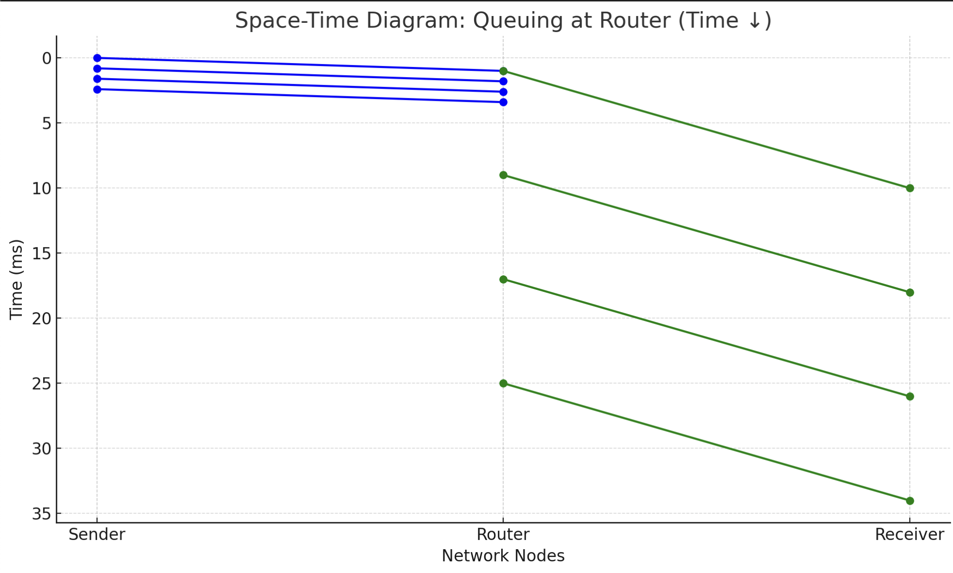
Notice how packets queue up at the router and experience increasing delays before reaching the receiver.
- Blue lines: Packets traveling from Sender to Router (fast link, low delay).
- Green lines: Packets leaving Router to Receiver (slow link, queuing occurs).
Scenario
The Sender sends 4 packets back-to-back at 10 Mbps. The Router receives them and forwards them one by one at 1 Mbps to the Receiver.
Answer the following questions:
- What is the transmission delay for each hop (Sender→Router, Router→Receiver)?
- When does each packet arrive at the router?
- When does each packet leave the router?
- What is the queuing delay at the router for each packet?
- When does each packet arrive at the receiver?
- What is the total time from first packet sent to last packet received?
Hints:
- Transmission delay = size ÷ bandwidth
- Propagation delay is fixed (1 ms per hop)
- Router sends packets sequentially: no overlap
- Queuing delay = wait time at router before transmission starts
Transmission delays:
- Sender → Router (10 Mbps): 8000 ÷ 10^7 = 0.8 ms
- Router → Receiver (1 Mbps): 8000 ÷ 10^6 = 8 ms
These departure and arrival times should be treated as *timestamps*.
Packet arrival times at router (consider transmission delay from the sender + propagation delay):
- Packet 1: 0.8 ms + 1 = 1.8 ms
- Packet 2: 1.6 ms + 1 = 2.6 ms
- Packet 3: 2.4 ms + 1 = 3.4 ms
- Packet 4: 3.2 ms + 1 = 4.2 ms
Packet departure times from router (since we add transmission delay from sender and count it as arrival time, we don't doubly count it in departure):
- Packet 1: 1.8 ms (no queue)
- Packet 2: 9.8 ms (queued behind Packet 1)
- Packet 3: 17.8 ms
- Packet 4: 25.8 ms
Queuing delays at router:
- Packet 1: 0 ms
- Packet 2: 9.8 - 2.6 = 7.2 ms
- Packet 3: 17.8 - 3.4 = 14.4 ms
- Packet 4: 25.8 - 4.2 = 21.6 ms
Arrival times at receiver:
- Packet 1: 1.8 + 8 + 1 = 10.8 ms
- Packet 2: 9.8 + 8 + 1 = 18.8 ms
- Packet 3: 17.8 + 8 + 1 = 26.8 ms
- Packet 4: 25.8 + 8 + 1 = 34.8 ms
Total time from first packet sent (0 ms) to last packet received:
- 34.8 ms
Packets Keep Coming, But Nobody’s Home (Yet)
Background
When a network interface card (NIC) receives packets, it transfers them into a fixed-size area in memory called a ring buffer. This buffer is managed by the operating system kernel and the NIC driver. The ring buffer works like a circular queue: each new packet is placed in the next available slot, wrapping around when it reaches the end. The OS must process and remove packets from this buffer before it fills. If the OS is delayed (for example, due to high CPU load or competing processes), the buffer can overflow, and new packets will be dropped.
The OS is notified of incoming packets using hardware interrupts, which trigger the driver to begin processing. To reduce overhead, the OS may use interrupt coalescing or polling mechanisms (like NAPI in Linux) that batch multiple packets before handling them. While this improves CPU efficiency, it can increase delay under bursty or high-throughput conditions. Even if the physical network link has plenty of capacity, performance can degrade if the OS cannot keep up with packet arrival, hence turning a fast network into a bottleneck.
Scenario
A server receives high-throughput traffic over a fast link. However, due to CPU contention, it cannot process packets immediately. As a result, the NIC ring buffer fills up and packet drops occur. Network performance monitoring shows a sudden spike in application-level latency.
Answer the following questions:
- Where does queuing happen inside the OS when receiving packets?
- What causes buffer overflow even when link capacity is sufficient?
- How does interrupt handling affect packet processing speed?
- Why does high CPU usage worsen network latency?
- What techniques help reduce or absorb incoming bursts?
Hints:
- The NIC uses a ring buffer in kernel memory
- Packet arrival rate can exceed processing rate
- Deferred interrupts or batching can help under load
- Buffer size and CPU availability determine responsiveness
- Drops occur when buffers fill before they are emptied
Queuing occurs in the kernel’s network receive path, particularly in the NIC ring buffer, which temporarily stores packets before they are processed by the OS.
Buffer overflow happens when packets arrive faster than the OS can remove them from the buffer. This is common under CPU load, where the network driver cannot run quickly enough to drain the queue.
Interrupts from the NIC notify the OS that data has arrived. However, if interrupts are too frequent, they consume too much CPU. The OS may coalesce interrupts (process in batches) to reduce load, but this adds latency.
When the CPU is busy with other tasks, it cannot process packets promptly. This increases time in the buffer, adds delay, and may lead to packet drops if the buffer fills before processing catches up.
To mitigate this, systems use larger buffers, interrupt moderation, and multi-core packet processing (e.g., RSS or NAPI). These techniques help absorb short bursts and improve throughput under load.
Bits on the Move with a Ticking Timeout
Background
Network delay has multiple components. Two fundamental types are:
- Transmission delay: the time to push all bits of a packet onto the wire. It depends on packet size and link bandwidth.
- Propagation delay: the time for a bit to travel across the link, regardless of size. It depends on distance and signal speed.
These two delays dominate in different contexts. In long-distance satellite links, propagation delay is high. In low-bandwidth links, transmission delay dominates. Measuring and comparing them helps explain unexpected latency.
Scenario
Two identical packets are sent: one across a 1 Mbps Wi-Fi link spanning 100 meters, and another across a 10 Gbps transcontinental fiber link (5000 km). Each packet is 1,000 bytes. Assume propagation speed is 2×10⁸ m/s.
Answer the following questions:
- What is the transmission delay for each link?
- What is the propagation delay for each link?
- Which delay dominates in each case?
- How would performance change with larger packet sizes?
- How can systems adapt based on which delay dominates?
Hints:
- Transmission delay = size ÷ bandwidth
- Propagation delay = distance ÷ speed
- Bytes must be converted to bits
- Delays affect buffering and timeout choices
- Applications may batch or pipeline data to reduce overhead
For the 1 Mbps Wi-Fi link: transmission delay = (1000 bytes × 8) ÷ 1,000,000 = 0.008 seconds = 8 ms.
Propagation delay = 100 ÷ (2 × 10⁸) = 5 × 10⁻⁷ seconds = 0.0005 ms. So transmission dominates.
For the 10 Gbps fiber link: transmission delay = (1000 bytes × 8) ÷ 10,000,000,000 = 0.0000008 seconds = 0.0008 ms.
Propagation delay = 5,000,000 ÷ (2 × 10⁸) = 0.025 seconds = 25 ms. So propagation dominates.
With larger packets, transmission delay becomes more noticeable on low-bandwidth links, but still negligible on high-bandwidth links. Long-distance transfers remain limited by propagation.
Systems adapt by pipelining data (sending multiple packets at once), tuning retransmission timeouts, or using protocols that tolerate latency. Understanding which delay dominates helps optimize throughput and responsiveness.
The Calm Before the Queue
Background
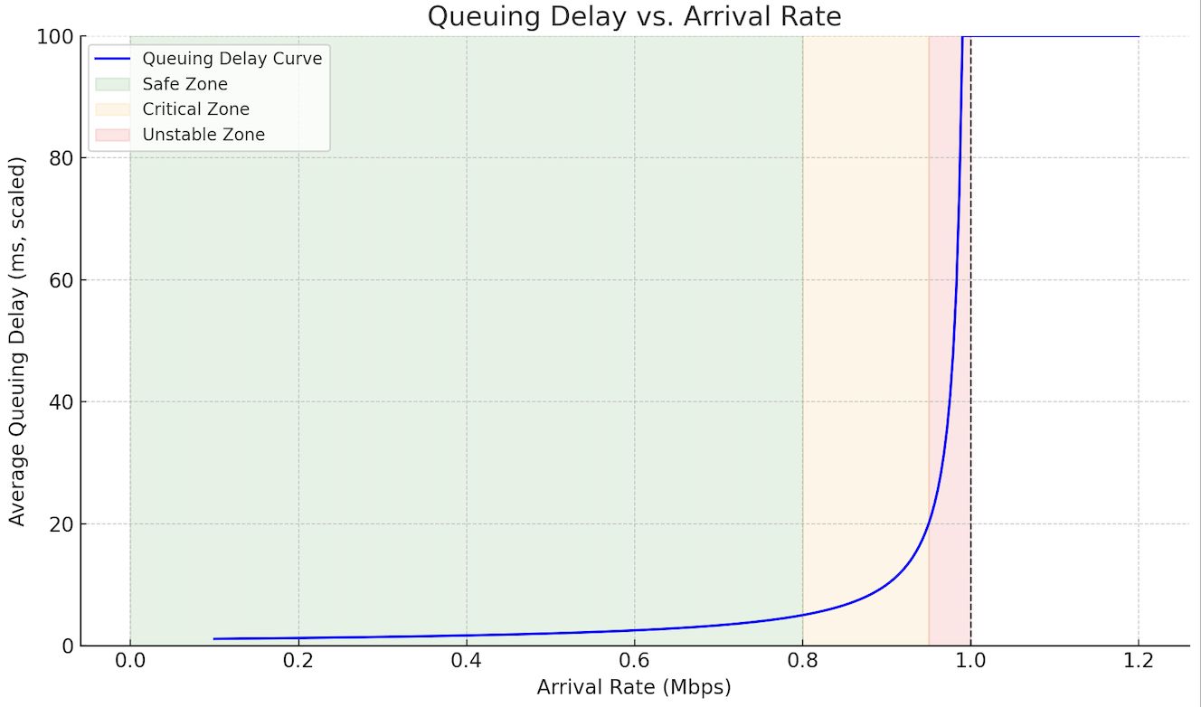
When packets arrive at a network device faster than they can be transmitted, they are queued in a buffer. As the arrival rate gets closer to the link transmission rate, the queuing delay increases. Slowly at first, then sharply. This relationship is non-linear: the delay remains low under light load but rises dramatically as the buffer nears capacity. Understanding this behavior helps explain why networks can feel suddenly “sluggish” even though they are not fully saturated.
Scenario
A router with a 1 Mbps output link handles varying traffic loads. As the average incoming rate increases from 0.1 Mbps to 1.2 Mbps, users notice occasional bursts of latency. This graph plots queuing delay (y-axis) versus traffic arrival rate (x-axis). The curve stays flat until about 0.8 Mbps, then increases steeply, especially near 0.95 Mbps:
Answer the following questions:
- Why is queuing delay low at low arrival rates?
- Why does delay grow rapidly near link capacity?
- What happens when the arrival rate exceeds the link rate?
- How does buffer size affect this curve?
- How could you design systems to handle traffic near capacity?
Hints:
- When arrival rate < link rate, the buffer empties faster than it fills
- Near full load, the buffer starts to build up
- Delay increases non-linearly as service time becomes critical
- Excess packets can be dropped when the buffer overflows
- Techniques like traffic shaping or early drop can manage this growth
At low arrival rates, the router can forward packets faster than they arrive. The buffer rarely builds up, so queuing delay stays near zero.
As arrival rate nears the link capacity, the router barely keeps up. Any small burst or variance causes packets to wait in the queue, increasing delay significantly.
When arrival rate exceeds link rate, **packets arrive faster than they can be sent**. The queue grows continuously, leading to long delays and eventually buffer overflow.
Larger buffers absorb bursts better but may increase delay under load. Smaller buffers reduce worst-case delay but increase risk of packet loss.
To manage traffic near capacity, systems can use Active Queue Management (e.g., RED), flow control, or delay-aware congestion algorithms that adjust sending rate before queues build up excessively.
The Idle Interface
Background: Link Utilisation Rate
Link utilization measures how effectively a network link is used. It is defined as the fraction of time the link is actively transmitting data, as opposed to being idle. Low utilization often means the link is underused, possibly due to long propagation delays, small packets, or bursty traffic. Even on high-bandwidth links, poor pipelining or application delays can cause the interface to spend most of its time waiting. Understanding utilization helps diagnose inefficiencies where the network is fast, but performance is still poor.
Scenario
A file transfer sends a single 1500-byte packet every 100 ms over a 10 Mbps link with negligible propagation delay. Students are asked to compute the link utilization and explain why the link feels “slow” despite low latency and decent bandwidth.
Answer the following questions:
- What is the formula for link utilization?
- How long does it take to transmit one packet in this case?
- What is the utilization over each 100 ms interval?
- Why does low utilization lead to underperformance?
- How could the system improve efficiency in this setup?
Hints:
- Utilization = transmission time ÷ total cycle time
- Transmission time depends on packet size and bandwidth
- Idle time dominates if packets are infrequent
- Small or infrequent sends waste bandwidth
- Batching or pipelining can raise efficiency
Link utilization is defined as the ratio of transmission time to the total time in a transmission cycle. It shows how much of the time the link is actually used.
The transmission time for a 1500-byte packet on a 10 Mbps link is (1500 × 8) ÷ 10,000,000 = 0.0012 seconds = 1.2 ms.
Each packet is sent once every 100 ms, so the utilization is 1.2 ÷ 100 = 0.012 or 1.2%.
Even though the link is fast, it is idle 98.8% of the time. This low utilization results in poor throughput, especially for large transfers, because most of the time is spent waiting between packets.
To improve utilization, the sender could send larger batches of packets at once, reduce spacing between transmissions, or use pipelined protocols that keep the link busy continuously.
The Overstuffed Switch
Background
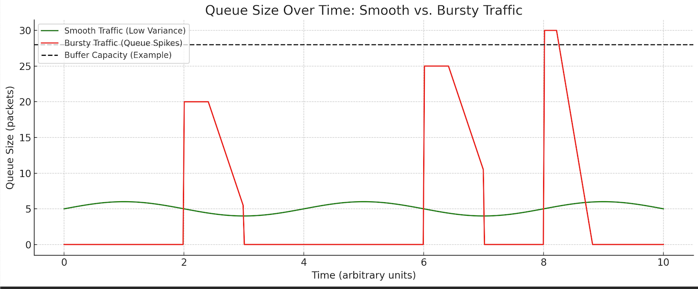
Network switches and routers buffer packets when arrival rate briefly exceeds link capacity. If traffic arrives in bursts, even if the average arrival rate is below capacity, queues can temporarily overflow. This leads to packet drops or increased delay. Queues are stable when the average service rate exceeds the average arrival rate over time. However, burstiness (short, high-volume spikes) can cause instability if the buffer is not large enough or the system is slow to respond.
The graph below illustrates the differences between bursty and smooth traffic, and how bursty traffic can trigger packet loss as the number of arriving packets exceed the router capacity:
Scenario
A switch receives two input streams. Each sends packets in large bursts, followed by idle gaps. The combined average arrival rate is below the link’s output capacity. However, the buffer occasionally overflows, and some packets are lost even though, on paper, the link should handle the load.
Answer the following questions:
- Why can a switch drop packets even if average arrival rate is below capacity?
- What role does burstiness play in queuing instability?
- How does buffer size influence packet loss in this case?
- What mechanisms help absorb bursts without loss?
- How can we balance delay and reliability in queue design?
Hints:
- Instantaneous arrival rate can exceed service rate
- Short-term overload fills the queue before it drains
- Larger buffers delay loss but increase latency
- Traffic shaping and pacing reduce burst impact
- Queue management must balance size and responsiveness
A switch can drop packets even if the average arrival rate is below capacity because packet arrivals are not evenly spaced. If many packets arrive in a short burst, the queue fills faster than the link can drain it.
Burstiness leads to temporary overload, where the buffer must absorb a sudden increase in traffic. If the burst is large enough and the buffer is small, packets will be dropped even though the average rate is sustainable.
A larger buffer can absorb more of the burst before overflowing. However, if the queue becomes too large, it introduces extra queuing delay for every packet.
Mechanisms such as traffic shaping, pacing, or active queue management (e.g., RED or CoDel) help smooth traffic and reduce the chances of burst-induced loss.
Effective queue design must balance reliability (avoiding drops) and latency (keeping queues short). Buffer size, link capacity, and traffic patterns all influence this balance.