Turing Machine

50.002 Computation Structures
Information Systems Technology and Design
Singapore University of Technology and Design

Turing Machine

Overview

A Finite State Machine does not keep track of the number of states it visited, it is only aware of the current state it is in. Therefore it is unable to solve problems like detecting palindrome or checking balanced parenthesis. There is no way to tell whether you have visited a state for the first time, or for the $n^{th}$ time.

A Finite Automata (FSM), cannot count.

The Turing Machine is a mathematical model of computation that defines an abstract machine: one that is able to implement any functionalities that FSM can implement, and it doesn’t face this limitation that FSM has.

Basics of Turing Machine

A Turing Machine is often represented as an “arrow” and a series of input written on a “tape”, as drawn in the figure below:

Turing Machine Basics :

The idea is to imagine that we have a physical machine (like a typewriter machine or something), called the Turing Machine, which can read a sequence of inputs written on an infinitely long “tape” (its basically an array).
We can write onto the currently pointed location of the tape (and also read from it).
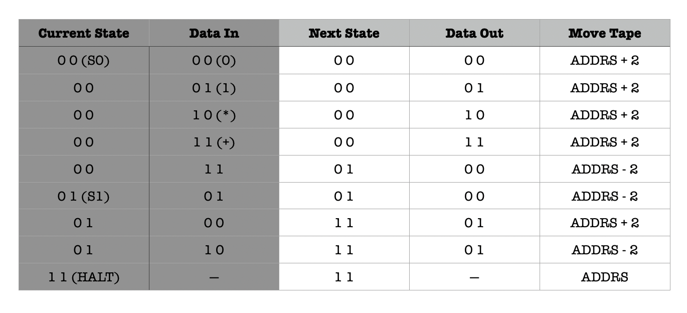
Like an FSM, the Turing Machine also has a specification, illustrated by the truth table above. Building a Turing Machine with specification $K$ allows it to behave based on $K$ when fed any array of inputs.
The pointer of the machine (black arrow) represents our current input read on the tape.
To operate the machine, we can move the tape left and right to shift the arrow, or you can move the arrow left and right. They are the same.

Note that in order to move the arrow to the right right, we need to equivalently move the tape to the left. In practice, we move the tape, not the arrow.
There exists a HALT state where you reach the end-state, and of course a START state as well.

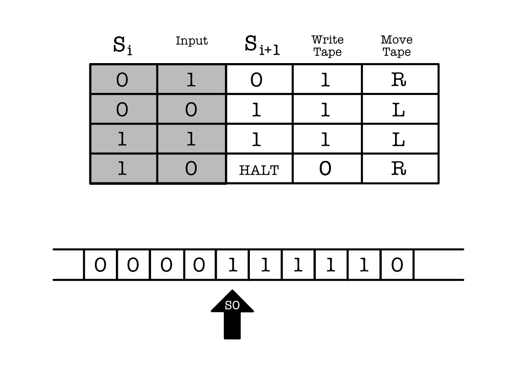
Turing Machine Operation :

Referring to the figure above, we know that the start state is $S_0$, and as shown the black arrow is reading an input: $1$
Then look at the functional specification table to know where to go next.
- From the diagram, our current state is $S_0$ and input is $1$. From the table, this corresponds to the first row – it tells us that we can write $1$ to the tape,
- And then move the tape to the right (or equivalently move the arrow to the left).
- It is important to write first, and then move the tape/arrow, not the other way around. So the sequence at each time step is: read-write-move.
Repeat step (1) and (2) until we arrive at a HALT state.
Depending on what we write onto the tape, we will end up with a different sequences on the tape when we reach step (3).

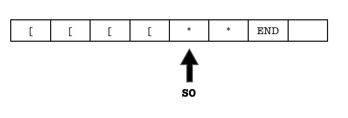
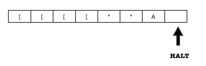
Example 1: Implementing an Increment Machine

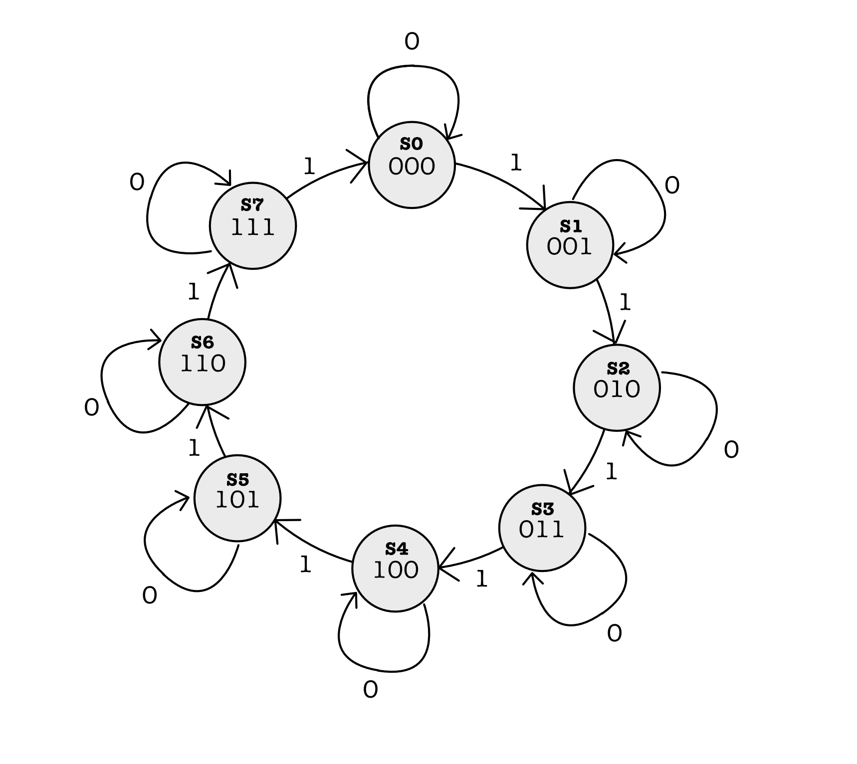
Consider a machine whose job is to add $1$ to any arbitrary length input and present that as the output. An FSM can do this as well if the number of bits of input is finite, but it will run into a problem if the input bit is too large. An example of a 3-bit counter FSM is:

The key feature for a Turing Machine is this infinite tape (hence its capability of processing arbitrary input).

A Turing Machine with the following specification can easily solve the problem and is capable to accept any arbitrarily long input with lesser number of states:

With this sample input, the Turing Machine runs as follows:

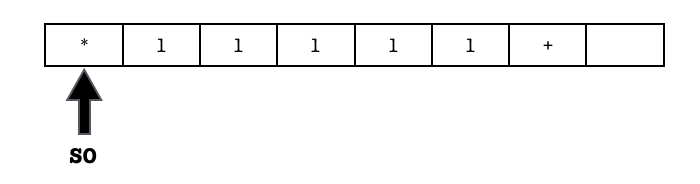
At t=0: The initial state of the machine is S_0, and the machine is currently reading $$ as an input (beginning of string). According to the first row of the table, it should write back a $$, and then move the tape to the left. In fact, the machine keeps moving the tape to the left until the end of the string (+) is found: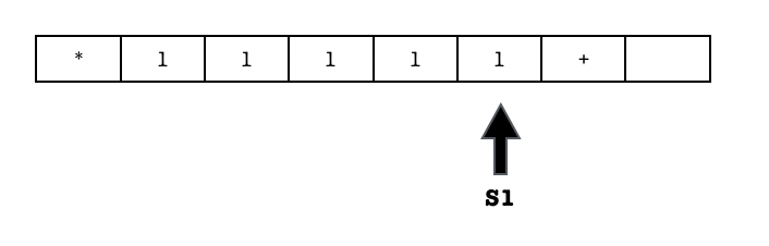
The machine then starts adding 1, and moving the tape to the right, keeping track of the carry over value:
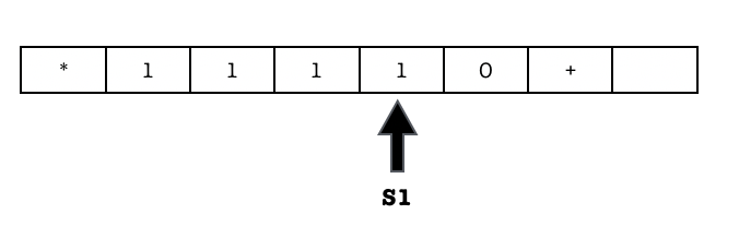
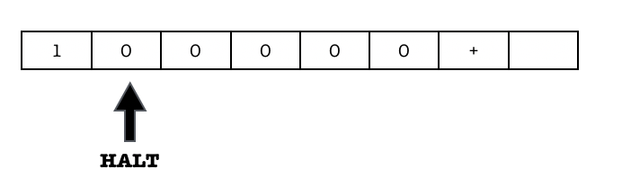
This continues until it reads back the beginning of the string (*):
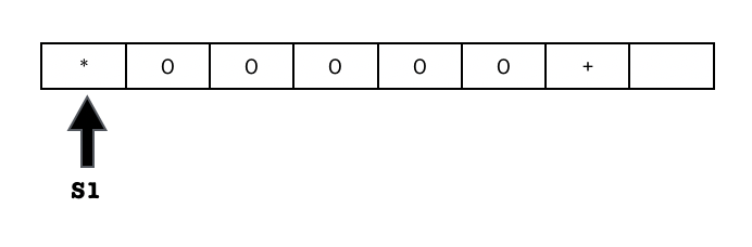
The final output is written on the tape, and we should have this output in the end when the machine halts:

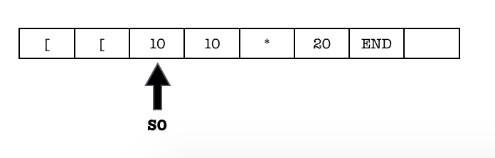
Example 2: Implementing a Coin Counter Machine

Suppose now we want to implement a machine that can receive a series of 10c coins, and then a series of 20c coins (for simplicity, we can’t key in 10c coins anymore once the first 20c coin is given). We can then press an END button in the end once we are done and the machine will:

ACCEPT (1) if the value of 10c coins inserted is equivalent to the value of 20C coins inserted, or
REJECT (0) otherwise.

A sample input will be:

10 10 10 20 20 20 20 END (REJECT)
10 10 10 10 20 20 END (ACCEPT)

For simplicity, an input as such 10 20 10 20 END will not be given (although we can also create a Turing machine to solve the same task with this input type, but the logic becomes more complicated).

We cannot implement an FSM to solve this problem because there’s no way an FSM can keep track how many 10s are keyed in so far (or 20s), and we can’t possibly create a state for each possible scenario,

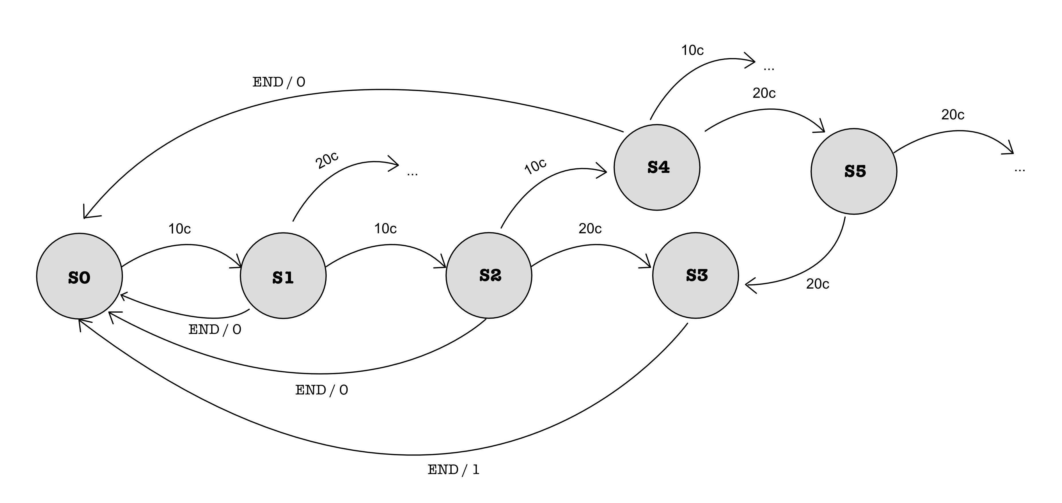
However, a Turing machine with the following specification can solve the problem:

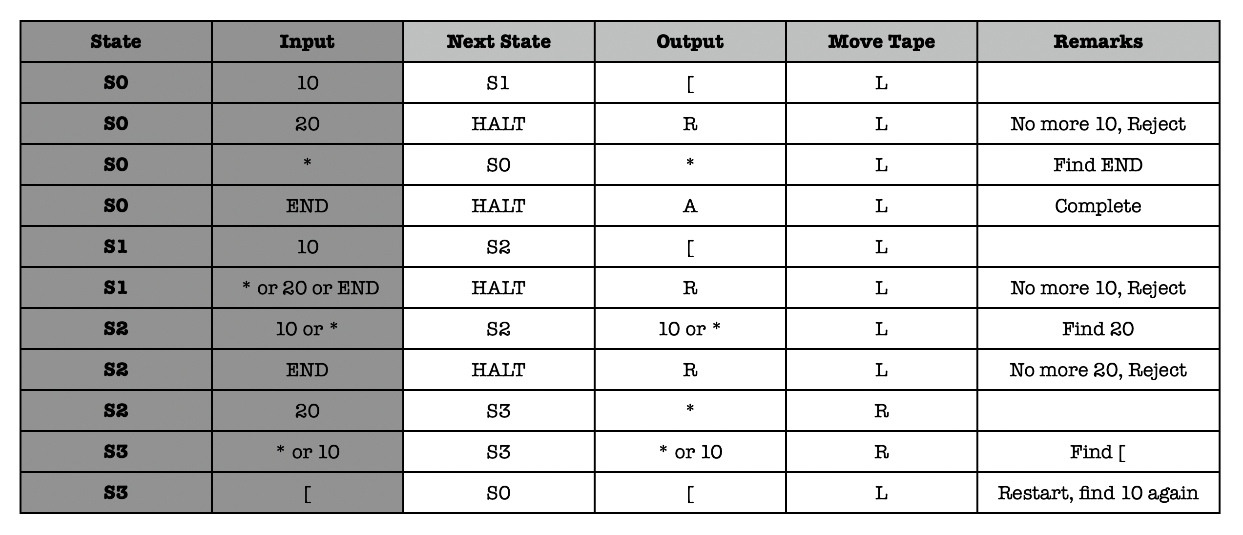
Given an input as follows and starting state at S_0 (at t=0):

The state of the machine is as follows at t=2:

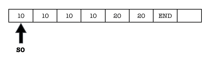
It will try to find the first ‘20’, and has this outcome and state at t=5 once the first ‘20’ is found:

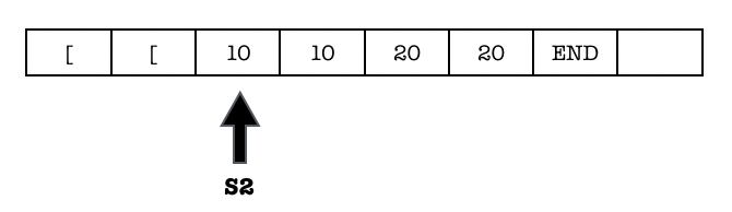
It will then try to find the leftmost unprocessed ‘10’:

The whole process is repeated until there’s no more 10. The Machine now will try to find END:

Once found, it halts and wrote the final value (ACCEPT):

As practice, you can try the running the machine using another set of input that will result in a REJECT.

Can you solve the problem with lesser states? Why or why not?

Turing Machine as a Function

Given a Turing Machine with a particular specification $K$ (symbolised as $T_K$), and a tape with particular input sequence $x$ (lets shorten it by calling it simply Tape $x$), we can define $T_K[x]$ as running $T_K$ on tape $x$,

We can produce $y = T_K[x]$, where $y$ is the output of a series of binary numbers on that corresponding Tape $x$ after running $T_K$ on $x$.
Running $T_K[x]$ therefore can be seen as calling a function that takes in input $x$ and produces output $y$.

Now the question that we need to address is, what kind of functions can Turing Machine compute? Or more generally, what can be computed and what type(s) of machines can compute them?

Church’s Thesis and Computable Function

The Church’s Thesis states that: Every discrete function computable by any realisable machine is computable by some Turing machine $i$.

So what is “computable function”?

Let’s look at some definition: “A function is computable if there exists an algorithm that can do the job of the function, i.e. given an input of the function domain it can return the corresponding output”. Any computable function can be incorporated into a program using while-loops.

What are the inputs to these functions?

In essence, anything discrete (integers):

A list of numbers $\rightarrow$ can be encoded large integer
A list of characters $\rightarrow$ also can be encoded a large integer
A matrix of pixels $\rightarrow$ also can be encoded a large integer
etc, you get the idea.

Hence whatever inputs $x$ we put at the tape, ultimately we can see them as a very large integer.

Can’t wrap your head around it? Look up ASCII encoding and try to translate “Hello World” into binary. You probably will get an output like: 01001000 01100101 01101100 01101100 01101111 00100000 01010111 01101111 01110010 01101100 01100100. Now convert this into decimal, its a very large integer isn’t it?

What are these “realisable” machines?

Any machine, there’s so many examples: any machine that help you sort, search, re-order objects, find maximum or minimum (of something), perform mathematical operations (multiply, add, comparisons, etc), the list goes on.

So what Church’s Thesis tell us is that there always exist a Turing Machine $i$ that can compute any function that is computable by any realisable (i.e: able to be achieved or happen, or any mechanical) machine.

Then, are there any uncomputable functions?

Just as there are infinitely many computable functions, there are also infinitely many uncomputable functions. Not every well-defined (integer) function is computable.

One of most famous example of uncomputable function is the Halting function $f_H(K,j)$, defined as:

\[\begin{aligned} f_H(K,j) = &1 \text{ if } T_K[j] \text{ halts}\\ &0 \text{ otherwise} \end{aligned}\]

In laymen term: the function determines whether Turing Machine that’s run with specification $K$ will halt when given a tape containing input $j$. What is “halt”? For example, we can write a program as an input to our machine (computers).

The program: print("Hello World") halts, while this program: while(True): print("Hello World") does not halt.

If $f_H(K,j)$ is computable, then there should be a specification $H$ that can solve this.

Lets symbolise a Turing machine with this specification as $T_{H}[K,j]$.

Now since there’s no assumption on what $j$ is, $j$ can be a machine (i.e: program) as well. So the function $f_H(K,K)$ should work as well as $f_H(K,j)$.

In laymen term: inputting a machine to another machine is like putting a program as an input to another program. Lots of programs do this: compilers, interpreters, and assemblers all take programs as an input, and turn it into some other program. Remember, $T_K$ is basically a Turing machine with specification $K$. We can have a Turing machine that runs with specification $K$ with input that is its own specification (instead of another input string $j$, symbolised as $T_K[K]$.

With this new information (and assumption that $f_H(K,j)$ is computable), lets define another specification $H’$ that implements this function:

\[\begin{aligned} f_{H'}(K) = f_{H}(K, K) = &1 \text{ if } T_K[K] \text{ halts}\\ &0 \text{ otherwise} \end{aligned}\]

Lets symbolise a Turing machine with this specification as $T_{H’}[K]$ (there’s no more $j$).

Finally, if we assume that $f_{H’}(K)$ is computable, then we can define another specification $M$ that implements the following function:

\[\begin{aligned} f_M(K) = &\text{loops forever} \text{ if } (f_{H'}(K)== 1) \\ &halts \text{ otherwise} \end{aligned}\]

A Turing machine running with specification M is symbolised as $T_M[K]$.

We have so many symbols now, let’s do some recap:

$K$ is an arbitrary Turing Machine specification, $T_K$ is a machine built with this specification.

$j$ is an arbitrary input

$H$ is the specification that “solves” the halting function: $f_H(K,j)$. $T_H$ is a machine built with this specification.

$H’$ is the specification that “solves” a special case of halting problem: $f_{H}(K,K)$, i,e: when $T_K$ is fed $K$ as input (instead of $j$). $T_{H’}$ is a machine built with this specification.

$M$ is the specification that tells the machine running it to loop if $f_{H’}$ returns 1, and halts otherwise. $T_{M}$ is a machine built with this specification.

In summary terms: $T_M$ loops if $T_K[K]$ halts (hence the output of $T_{H’}[K]$ is 1), and vice versa.

Now since $K$ is an arbitrary specification, we can make $K=M$, and fed the function $f_M$ with itself:

\[\begin{aligned} f_M(M) = &\text{loops forever} \text{ if } (f_{H'}(M)== 1) \\ &halts \text{ otherwise} \end{aligned}\]

Don’t worry, we are almost at the end of our proof.

Running $T_M[M]$ will call these chain of events. We explain it in terms of “function calls” instead of Turing machine running (although they are equivalent) because it may be easier to understand:

When we call $f_M(M)$ (running $T_M[M]$), it needs to call $f_{H’}(M)$ (run $T_{H’}[M]$) because it depends on the latter’s output

$f_{H’}(M)$ depends on $f_H(M,M)$: the original halting function that outputs 1 if $T_M[M]$ halts, and 0 otherwise.

That means, we need to call $f_H(M, M)$ to find out its output, so that $f_{H’}(M)$ can return.

Calling $f_H(M, M)$ requires us to run a Turing Machine with specification $M$ on input $M$ (run $T_M[M]$ for another time), identical with what we did in step (1) above (just like recursive function call here).

Now here is the contradiction:

If the running of $T_M[M]$ from step (4) halts, then it will cause $T_{H′}[M]$ to return $1$. If $T_{H′}[M]$ returns 1, then the running of $T_M[M]$ from step (1) loops forever.
But, if the running of $T_M[M]$ from step (4) loops forever, then it will cause $T_{H′}[M]$ to return $0$. If $T_{H′}[M]$ returns 0, then the running of $T_M[M]$ from step (1) halts.

Neither can happen.

Therefore, specification $M$ does not exist and it is not realisable. And by extension, everything falls apart: specification $H’$ and $H$ do not exist either. This means that $f_H(K,j)$ is not computable.

Universal Function

The universal function is defined as:

\[f_{U}(K,j) = T_K[j]\]

Let’s say we can write a specification $U$ that realises this function.

This means that a Turing Machine that runs $U$ is a Turing machine that is capable of simulating an arbitrary Turing machine on arbitrary input. This is called a Universal Turing Machine.

The universal machine essentially achieves this by reading both the specification of the machine $K$ that we are going to simulate as well as the input $j$ to that machine from its own tape.

A more familiar term for this “specification” is simply a program.

The universal function is a model of general purpose computer. Our computers are essentially a machine that simulates other machine: it is a calculator, a gaming console, a video player, a music player, a telephone, a chatting device, and many others.

Most importantly: our computer can emulate and be any machine when we task it to run any program and its input. It can be a text editor, video game emulator, video player, music player, radio, telephone, camera, and many more.

Summary:

Back to the notion of universal function $U$ above, it has two inputs $K$, and $j$. Let’s build a Turing machine with this specification, and symbolise it as $T_U(K, j)$.
The “specification” $K$ is basically a program that specifies which computable functions we want to simulate.
$j$, is the data tape $T_K$ is going supposed to read.
We can create a Turing Machine $K$ to run on input $j$: $T_K[j]$, but of course this machine $T_K$ can only perform function $K$.
Meanwhile, $T_U$: our universal machine, interprets the data, $K$ and $j$ is capable of emulating the behavior of $T_K[j]$ (without having to build $T_K$).
Therefore with $T_U$, we no longer need to make any other Turing Machine $T_K$ that can only compute function $K$, because $T_U$ can emulate the behavior of any Turing Machines

The closest actual realisation of $T_U$ is basically our general purpose computer. It can run programs and perform it just as intended. We can simply write any new program $K$, and execute it on $T_U$ using some input $j$.

We no longer need different machines to: watch TV shows, listen to music, and chat with our friends. We just need our computer to do all the three different tasks.

Where is that “infinitely long tape” in our computers?

Well, technically, our computers have a very long tape (i.e: its memory), where its programs and inputs (and outputs) are stored. It is large enough to make us feel like it is infinite when it is not. By definition, computer can in fact be realised using FSM (not strictly a Turing Machine because infinitely long Tape doesnt exist), just that we probably need billions of state to do so.

Summary: The Computer Science Revolution

Imagine the hassle and inconvenience if we need to build a different physical machine $T_M$ each time we need to compute a new function $f_M$.

For example, suppose we want to make a physical machine that can perform sorting where it receives an array of integer as an input.

We probably need other “simpler” (physical) machines that can perform comparison, addition, shifting, etc because all these parts are required to do the former tasks. This is very complex to do as we have many things to consider:

How do we connect these machines together? Do we solder thousands of wires manually?
How big or heavy, or costly is this final machine going to be?
If we need to add or compare $N$ terms together, how many “adder” machines do we need? Can we reuse them? Or do we order $N$ duplicates of these physical adder machine?

In order to be efficient, we need to replace each of these hardwares with a coded description of that piece of hardware (i.e: a software), then its easy to cut, change, mix, and modify them around. Writing a merge-sort algorithm is so much easier (instead of building a physical machine that can perform sorting). Also, programs can easily receive another program as input and output other programs.

This is the universal Turing Machine: a coded description of a piece of hardware. It allows us to migrate from hardware paradigm into software paradigm. People are no longer spending their time sitting in workshops making physical systems but they are now sitting in front of computers writing programs.

Until this point, we have learned how Turing machine works, and its advantage over FSM. Our final goal is to realise a Universal Turing machine, that is a machine that is programmable so that it can be used for a general purpose.

Programmability

The concept of a universal Turing Machine is an ideal abstraction, since we can never create a machine with infinitely long tape. However, physically creating something that is “infinite” is not possible.

We can only create a very long “tape” such that it appears “infinite” to some extent.

If we manage to create a physical manifestation of Universal Turing Machine, we need to ensure that this machine is programmable. This can be achieved by designing an instruction set so that we can write “programs” / “algorithms” using these instruction set.

Hence allowing it to emulate the behavior of whatever machine $k$ when running the program with its corresponding input $j$ on this machine.

An instruction set is a set of standard basic commands that we can use as building blocks so that we can write a bigger programs that will cause the machine running it to emulate complex tasks.

For example:

We are familiar with high level programming languages, such as C/C++, Java, and Python. You can write a program using any of these languages, lets say a calculator app. When we compile or interpret, and then run the program, our code is translated into a set of instructions that are understandable by our machine, hence turning it into a calculator.
We can also write another program, lets say a music player app. When we run this program, our computer turns into a music player.

Therefore, we can say that our computer is programmable, because the program that we wrote is translated into a set of instructions that our machine can understand.

Our (general purpose) computer is a (close enough) physical manifestation of a Universal Turing Machine (albeit with “finite” tape).

In the next chapter, we will learn further on how our general purpose computer is programmable by designing a proper instruction set for it.

Appendix: Sample Manifestation of a Turing Machine

This section tells us one of the ways to realise the incrementer Turing Machine sample above as an actual machine using hardware components that we have learned in the earlier weeks.

First, we need to encode the logic of the machine in terms of binary values. We can use 2 bits to represent the state: S_0, S_1, and HALT and 2 bits to represent the input/output characters: 0, 1, * and + each.

We also must create a kind of addressable input tape (memory unit that stores the data). Imagine that we can address each bit in the input tape as such, where ADDRS is an n-bit arbitrary starting address:

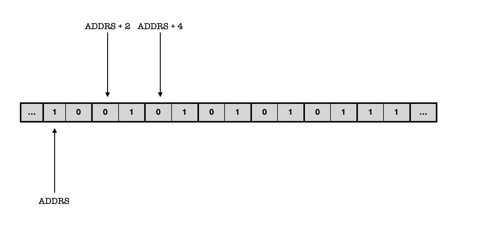
Since we want to read and write two bits of input and output at a time (i.e: at each clock cycle), we can “move the tape” by advancing or reducing the value of Current Address (that we supply to the addressable memory unit) by 2 at each clock cycle.

Note: it is impossible to have “infinitely large” memory unit, so in practice we simply have a large enough memory unit such that it appears infinite for the particular usage.

We can then construct some kind of machine control system (the unit represented as the arrow in the TM diagram). This similar to how we build an FSM using combinational logic devices to compute the TM’s 2-bit output data, next address, and the next state, given current address, current state, and 2-bit input data based on the functional specification stated in the truth table above.

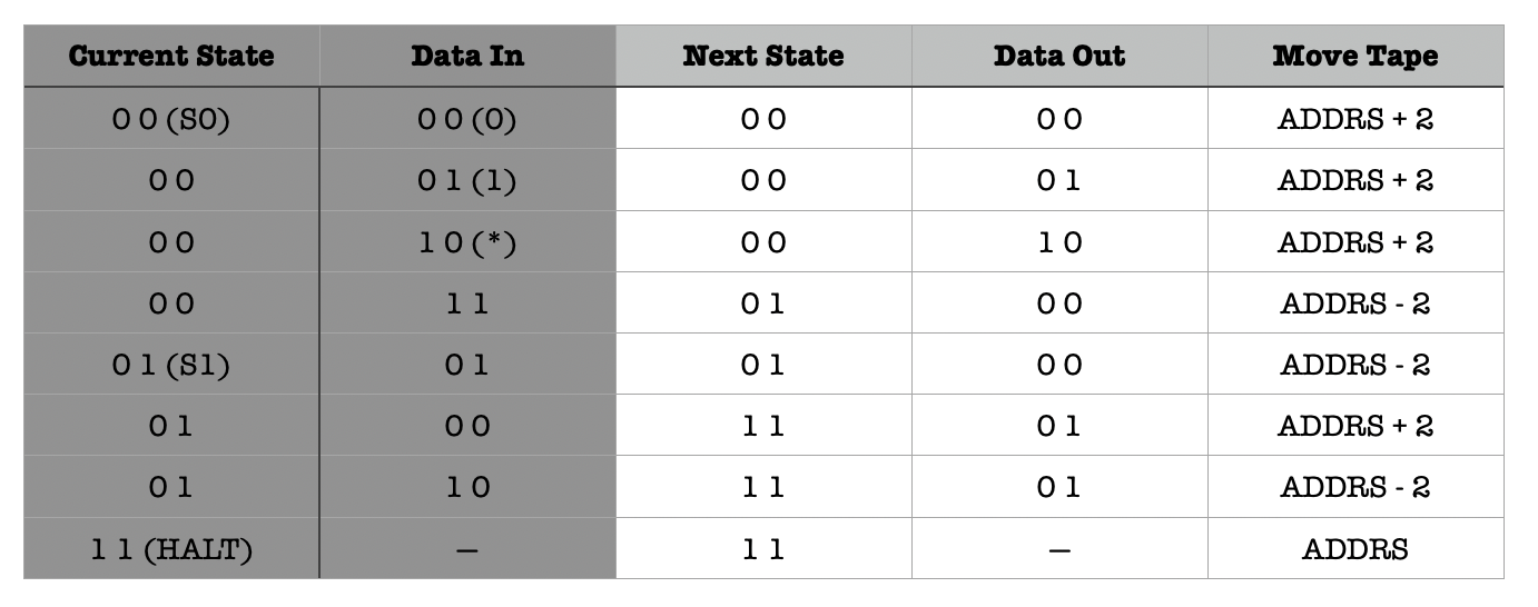
The diagram above shows a rough schematic on how we can realise the abstract concept of a Turing Machine with a specification that does increment by building a (non-programmable) physical machine that can only do this one task.